Home/Analysis Technologies/Electromagnetic analysis/FEEM

Analysis Technologies | Electromagnetic Analysis

FEEM (Finite-Element Eigenmode)

A method that divides the cross-section of a structure uniform along the propagation direction into triangular finite elements and solves an eigenvalue problem for the propagation constant and field profile of each mode.

Discretization

Triangular finite-element mesh

Problem solved

Two-dimensional eigenvalue problem on the cross-section

Supporting products

Lumerical Multiphysics

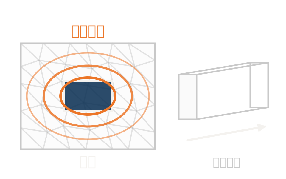
Schematic of the cross-section of a waveguide uniform along the propagation direction, with the mode field distributed over it

What the method is

Solving the modes as a cross-sectional eigenvalue problem

Assuming the structure is uniform along the propagation direction, the fields can be written as the product of an in-plane distribution and a term whose phase advances along that direction. That assumption reduces Maxwell’s equations to a two-dimensional eigenvalue problem on the cross-section, with the propagation constant as the eigenvalue and the mode field profile as the eigenvector.

The cross-section is divided into triangular elements. The maximum triangle edge length is set relative to the free-space wavelength, and refinement can be specified by material or region. The polynomial order of the basis functions used on the elements is also selectable.

The effective index follows from the propagation constant and the angular frequency. For lossy materials, propagation loss follows from the imaginary part of the effective index. Each mode field is normalized so that it carries 1 W of power.

How it works

Use the uniformity along the propagation direction, and solve as a cross-sectional eigenvalue problem

The method presumes the structure is uniform along the propagation direction. Under that premise the fields can be written as the product of an in-plane distribution and a term whose phase advances along the propagation direction, so a three-dimensional problem becomes a two-dimensional one on the cross-section. The finite-element method discretizes that as a generalized eigenvalue problem over triangular elements covering the cross-section. The eigenvalue corresponds to the square of the effective index, and the solution comes as a discrete set of modes.

Finite-element formulations for vector fields have an intrinsic difficulty: unphysical spurious solutions appearing in the numerical spectrum. Using edge elements for the transverse components and nodal elements for the longitudinal component is a widely used way of representing hybrid modes accurately while suppressing spurious solutions. This is a general property of the method.

DiscretizationThe cross-section is divided into triangular elements, and within each element the fields are expanded in vector basis functions of the specified order.
FormulationBecause of the assumed uniformity along the propagation direction, Maxwell’s equations become a generalized eigenvalue problem on the cross-section. The eigenvalue corresponds to the square of the effective index, giving the propagation constant, and the eigenvector gives the mode field profile.
Selecting the solutionsSolutions come as a discrete set of modes. You have to give the number of modes to find and the effective index to search around.
Accuracy controlAccuracy is set by both the triangle density and the polynomial order of the basis functions. For geometry with no curved surfaces, raising the order is often the more effective route.

Strengths of this method

Why this method is chosen

Following the geometry

An unstructured triangular mesh can be laid out along material interfaces. Where an orthogonal-grid solver is at a disadvantage on non-rectangular cross-sections, this represents complex boundaries as they are.

Suppressing spurious solutions

Edge-element formulations greatly reduce unphysical spurious solutions and are the standard in computational electromagnetics.

Accuracy through order

Rather than refining the mesh, you can raise accuracy by increasing the polynomial order of the basis functions.

Where it fits

Where it fits, and where it does not

Where it is a good fit

→ when you need the effective index, loss or effective area of a guided mode from the cross-section of a structure uniform along the propagation direction

→ when you want to quantify leakage into a high-index substrate using PML boundaries

→ when you want the modes of a bent waveguide at a specified bend radius

→ when you want to re-solve the modes with an index change obtained from thermal or electrical analysis applied

→ when you need effective index and group index to pass to circuit simulation

Where another method is the better fit

Structures not uniform along the propagation direction: the method assumes the form of an in-plane distribution multiplied by a phase term along the propagation direction. Devices whose shape changes along that direction are out of scope.

Three-dimensional scattering and radiation: if you need whole-device scattering or radiation rather than modes, you need a method that discretizes the analysis region as a volume.

Simple, near-rectangular cross-sections: if the cross-section is naturally represented on an orthogonal grid, orthogonal-grid mode analysis is sufficient. The capability to obtain group delay and dispersion in one go from a frequency sweep is on that side too.

When you want wavelength dependence in one go: modes are solved one frequency at a time. Quantities such as group index are obtained by computing at several wavelengths.

Applications

Typical applications

Silicon photonics waveguides

Obtain the mode profile, effective index, loss, TE and TM fractions and effective area of an SOI waveguide.

Leakage loss into the substrate

Use PML boundaries to obtain the fraction radiated into a high-index substrate as loss.

Thermo-optic phase shifters

Convert the temperature distribution from a thermal analysis into an index change and obtain the phase change against input power.

Parameter extraction for a circuit model

Obtain effective index and group index and pass them to the waveguide element in circuit simulation.

Inputs and outputs

What you provide, and what you get

INPUT

Cross-sectional geometry Combinations of primitives, the layer builder, and import from GDSII, STL or STEP
Material Refractive index data. An index change obtained from an external analysis can also be applied
Analysis conditions Wavelength or frequency, the number of modes to find, the effective index to search around, and the bend radius for a bent waveguide
Mesh Edges per wavelength, polynomial order of the basis functions, minimum triangle angle

OUTPUT

Effective index and loss Propagation constant and effective index per mode, and propagation loss (dB/m)
Mode profile Distributions of electric field, magnetic field and Poynting vector on the cross-section
Mode properties TE and TM polarization fractions, and effective area
Mesh information Node coordinates, element connectivity and polynomial order

How it works

How it works in practice

01

Define the materials

Define the materials that make up the cross-section, such as core, cladding and substrate.

02

Build the cross-section and assign materials

Build the cross-section of a structure that can be taken as uniform along the propagation direction and assign the materials you defined.

03

Settle the analysis region and mesh

Set the analysis region and settle the edges per wavelength and the polynomial order. The defaults are 1 edge and order 3.

04

Solve the modes and evaluate

Give the wavelength, the number of modes to find and the effective index to search around, run the calculation, and evaluate effective index, loss, polarization fractions and effective area.

The default settings are coarse. In an Ansys example, raising edges per wavelength to 5 and polynomial order to 10 brought the difference from the reference value to within 0.005%. Vary refinement and order and confirm the point at which the result stops moving.

Comparison with related methods

Choosing between related analysis methods

Method Relationship Main targets When to use which
FEEM (this method) This method Cross-section of a structure uniform along the propagation direction Divides the cross-section into triangular finite elements and solves an eigenvalue problem for the propagation constant and field profile of each mode. Each mode is normalized to carry 1 W of power.
FDE Alternative Cross-sections representable on an orthogonal grid Solves the same cross-sectional eigenvalue problem on an orthogonal grid. Normalization is to a peak electric field intensity of 1, and it has a frequency sweep capability.
DGTD Complementary Three-dimensional structures with curved surfaces Also finite-element, but solves the three-dimensional Maxwell equations in the time domain.
FDTD Complementary Three-dimensional structures at wavelength scale Discretizes the analysis region as a volume and gives spectra, far fields and S-parameters.

View all analysis technologies →

Supporting products

Products that provide this method

A commercial software environment providing finite-element eigenmode analysis. Charge transport, heat transport, multiple quantum well and three-dimensional electromagnetic solvers sit in the same environment, so thermal and electrical results can be carried into the mode analysis. See here for licensing, system requirements and deployment.

Lumerical Multiphysics

View the product page →

FAQ

Frequently asked questions

How does this differ from orthogonal-grid mode analysis?The quantities obtained are similar, but the discretization differs. Triangular finite elements can be laid out along material interfaces, so the further the cross-section departs from rectangular, the more the two differ. The normalization convention also differs: here each mode is normalized to carry 1 W of power.
How many modes can it find?You specify the number of modes to find. Alongside that, give either the effective index to search around or the setting that searches near the maximum index in the mesh. Mode selection is not automatic.
Is there a guide to mesh settings?The defaults are 1 edge per wavelength and polynomial order 3. In an Ansys example, 5 edges and order 10 brought the difference from the reference value to within 0.005%. For geometry with no curved surfaces, raising the polynomial order is considered more effective than refining the mesh.
Can it give leakage loss into the substrate?Yes. With PML boundaries, the fraction radiated into a high-index substrate can be obtained as loss. That boundary condition was added in release 2021 R1.4.

References

Last updated

2026-08-18

Technical review

LightBridge Technical Support

Sources consulted

Ansys Optics: Finite Element EigenMode (FEEM) solver introductionAnsys Optics: FEEM solver – Simulation objectAnsys Optics: FEEM product reference manualAnsys Optics: Waveguide (FEEM)Ansys Optics: Waveguide Substrate Loss (FEEM)Ansys Optics: Thermally tuned waveguide (FEEM)

We can advise on mode analysis of waveguide cross-sections

Tell us the cross-sectional structure and the characteristics you want to evaluate, and we will propose the method and product that suit.