
Home/Analysis Technologies/Electromagnetic analysis/DGTD

Analysis Technologies | Electromagnetic Analysis

DGTD (Discontinuous Galerkin Time-Domain)

An electromagnetic method that solves Maxwell’s equations in the time domain. Because it uses an unstructured mesh of triangles or tetrahedra, curved and slanted interfaces can be represented in their true shape.

Discretization

Unstructured mesh (triangles and tetrahedra)

Accuracy control

Mesh density and polynomial order

Supporting products

Lumerical Multiphysics
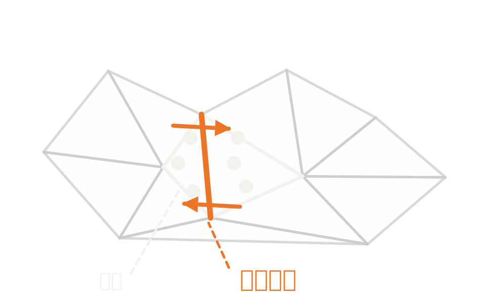
Schematic of a region divided into triangular elements, showing two neighboring elements coupled by the numerical flux across the face they share

What the method is

Expand the fields within each element, join them at the faces

The analysis region is divided into an unstructured mesh of triangles (2D) or tetrahedra (3D), and within each element the electric and magnetic fields are expanded in polynomials up to a specified order. Because elements can follow the geometry, curved and slanted interfaces need no staircase approximation.

It is a time-domain method, stepping Maxwell’s equations explicitly for isotropic, dispersive, non-magnetic materials. Relative permittivity given in the frequency domain can also be handled.

Accuracy can be raised not only by refining the mesh but by increasing the polynomial order. Raising the order also raises the cost, so how you divide effort between the two is the key to the setup.

How it works

Approximate the fields independently in each element, couple them by numerical flux at the faces

In the discontinuous Galerkin method the fields are approximated independently element by element. Within each element they are represented by polynomials of the specified order, and the approximations in neighboring elements do not necessarily agree at the shared face. What may be discontinuous is the numerical representation, not the physical quantity. Elements exchange information through a numerical flux term on the face.

That formulation keeps most of the arithmetic inside the elements and makes the mass matrix block diagonal. Because each element can be inverted on its own, explicit time stepping is affordable. The division into elements is also the division used for parallel computation.

DiscretizationThe analysis region is divided into an unstructured mesh of triangles or tetrahedra, and within each element the fields are expanded in polynomials of the specified order.
Coupling between elementsEach element’s approximation is independent and is tied to its neighbors only by the numerical flux term at the face. What is allowed to be discontinuous is the per-element numerical representation, and most of the arithmetic closes inside the element.
Time steppingTime stepping is explicit. There is an upper bound on the time step, set by the smallest element size and the polynomial order.
Accuracy controlAccuracy is set by both mesh density and polynomial order. Raising the order lets a coarse mesh represent rapid variation in the field.

Strengths of this method

Why this method is chosen

Following the geometry

An unstructured mesh can be laid out to follow any geometry, so curved and slanted interfaces are represented as they really are.

High-order accuracy

High-order basis functions and an unstructured mesh allow high-order discretization in space and time. That does not mean it is always more accurate or faster than FDTD: the choice of method comes down to the balance between geometric fidelity and the cost of meshing and computation.

Suits parallelization

Because arithmetic closes inside the elements and coupling is limited to the faces, it suits parallel computation by domain decomposition at element level.

Where it fits

Where it fits, and where it does not

Where it is a good fit

→ when the geometry does not follow an orthogonal grid and curved or slanted interfaces govern the behavior

→ when you want the resonant wavelength, Q factor and mode profile of a metallic nanostructure from a time-domain calculation

→ when you want to pass the absorbed optical power distribution to a thermal analysis as a heat source

→ when you want accuracy from a coarse mesh with high polynomial order rather than a fine uniform mesh

Where another method is the better fit

Geometry that follows an orthogonal grid naturally: if the geometry follows an orthogonal grid, the advantage of an unstructured mesh is not realized. The choice comes down to the balance between geometric fidelity and the cost of using an unstructured mesh.

Media that are anisotropic or magnetic: the materials documented for this method are isotropic, dispersive and non-magnetic. Anisotropic or magnetic media are out of scope.

Waveguide cross-sectional modes: if you want the modes of a structure uniform along the propagation direction, a method that solves the two-dimensional cross-sectional eigenvalue problem suits better.

Excitation other than a plane wave or Gaussian beam: the sources listed in the product reference are plane wave and Gaussian beam. If other excitation is needed, consider a method with a wider range of source types.

Applications

Typical applications

Plasmonic resonators

Obtain the resonant wavelength, Q factor and mode profile of a metallic nanostructure from a time-domain calculation.

Diffraction gratings

Solve a diffraction grating on an unstructured mesh and obtain efficiency by projection onto diffraction orders.

Optically induced heating

Take the absorbed power distribution from an absorption monitor as a heat source and carry it into a temperature analysis.

Scattering by small particles

Obtain the scattering and absorption cross-sections of spheres and small particles.

Inputs and outputs

What you provide, and what you get

INPUT

Structure Combinations of primitives, the layer builder, the dataset builder, and definition by formula
Material Isotropic, dispersive, non-magnetic materials. Plasma (Drude), Debye and Lorentz models, with automatic fitting to measured (n,k) data
Mesh and order Elements per wavelength and the polynomial order of the basis functions. The default is about 2 elements per shortest wavelength in each material
Sources and boundary conditions Plane wave or Gaussian beam. PML, absorbing, periodic, PEC and PMC boundary conditions

OUTPUT

Electromagnetic field distribution Electromagnetic fields on the mesh, from frequency and time monitors
Absorbed power The absorbed power distribution from an absorption monitor. It can be passed to a thermal analysis as a heat source
Cross-sections and resonant characteristics Extinction, scattering and absorption cross-sections, and the resonant wavelength and Q factor extracted from the time-domain waveform
Far field and diffraction orders Far-field projection from the near field, and projection onto diffraction orders for periodic structures

How it works

How it works in practice

01

Define the materials

List the materials used in the analysis and give their optical, electrical and thermal properties.

02

Build the geometry and assign materials

Create the geometric objects and assign the materials you defined. The advantage of an unstructured mesh shows on structures with curved or slanted surfaces.

03

Place the analysis region and solver, and settle the mesh

Decide the extent of the analysis, add the solver, and set how effort is divided between accuracy and cost using elements per wavelength and polynomial order.

04

Set sources, monitors and boundary conditions, and run

Place the solver-specific objects, check the errors and warnings, then run and evaluate the results returned.

Setting up a finite-element analysis follows a considerably different flow from FDTD or MODE. The default mesh is about 2 elements per shortest wavelength in each material, and in most cases refinement of specified regions or surfaces is required.

Comparison with related methods

Choosing between related analysis methods

Method Relationship Main targets When to use which
DGTD (this method) This method Structures with curved or slanted interfaces Represents geometry with an unstructured mesh and high-order basis functions and solves Maxwell’s equations in the time domain.
FDTD Alternative Geometry that follows an orthogonal grid Also time domain, but on an orthogonal grid. Its accuracy is set by points per wavelength, while this method also controls it by polynomial order. Neither is always the better choice.
FEEM Complementary Cross-section of a waveguide uniform along the propagation direction Also finite-element, but solves the two-dimensional cross-sectional eigenvalue problem and returns modes.
RCWA Alternative Layered structures with in-plane periodicity A semi-analytic method specialized to structures where periodicity can be assumed. If diffraction efficiency is the aim, it has the advantage in run time.
STACK Alternative Reflection and transmission that close within a layer stack An analytic method. Reflection and transmission of a plane multilayer are fully covered by it.

View all analysis technologies →

Supporting products

Products that provide this method

A commercial software environment providing electromagnetic analysis by the discontinuous Galerkin time-domain method. Waveguide mode analysis, charge transport, heat transport and multiple quantum well solvers sit in the same environment, so analyses can be combined. See here for licensing, system requirements and deployment.

Lumerical Multiphysics

View the product page →

FAQ

Frequently asked questions

Should I choose this or FDTD?As methods, the difference is how geometry is represented. An orthogonal grid is simple and efficient when the geometry follows it; an unstructured mesh represents curved and slanted interfaces as they really are, at the cost of meshing and computation. Neither is always the better choice. Talk to us about a comparison on your actual structure.
Is it better to refine the mesh or raise the polynomial order?Raising the polynomial order lets a coarse mesh represent rapid variation in the field, but it also raises the cost. The default mesh is about 2 elements per shortest wavelength in each material, so first check whether refinement of specified regions or surfaces is needed.
Why does a power monitor return two values?Because the field approximation is independent element by element and need not agree at element boundaries, a power monitor returns two values, computed on the front and back of the monitor surface.
Can it be coupled with thermal analysis?Yes. Passing the absorbed power distribution from an absorption monitor to a thermal analysis as a heat source is published as an example of optically induced heating of a metallic antenna.

References

Last updated

2026-08-18

Technical review

LightBridge Technical Support

Sources consulted

Ansys Optics: Discontinuous Galerkin Time-Domain (DGTD) solver introductionAnsys Optics: DGTD solver – Simulation objectAnsys Optics: Boundary conditions in DGTD – Simulation ObjectAnsys Optics: DGTD product reference manualAnsys Optics: Plasmonic resonator (DGTD)Ansys Optics: Photothermal heating in plasmonic nanostructures (DGTD)

We can advise on electromagnetic analysis of curved geometry

Tell us the geometry and the characteristics you want to evaluate, and we will propose the method and product that suit.