
Home/Analysis Technologies/Electromagnetic analysis/FDTD

Analysis Technologies | Electromagnetic Analysis

FDTD (Finite-Difference Time-Domain)

An electromagnetic method that solves Maxwell’s equations directly in the time domain. Space is divided into a grid and the electric and magnetic fields are updated alternately, so a single run yields a broadband response.

Discretization

Orthogonal grid (Yee cell)

Domain

Time domain, broadband

Supporting products

Lumerical FDTD
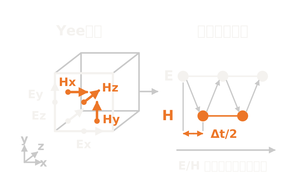
Schematic showing electric and magnetic fields staggered in both space and time on the Yee grid, updated alternately by half a step

What the method is

Discretize space and time, and solve directly

The analysis region is divided into an orthogonal grid, with the components of the electric and magnetic fields placed at slightly different positions within each cell and updated alternately through time. It discretizes Maxwell’s curl equations in space and time and solves them directly, introducing no modeling approximation into propagation or scattering. The discretization itself is a source of error, though, so the accuracy you get depends on the settings.

Fourier transforming the fields obtained in the time domain gives frequency-domain quantities such as the complex Poynting vector, transmittance and reflectance. That is why a single run yields the response over a wide wavelength range.

The grid is generated automatically, with finer cells in high-index and strongly absorbing materials. The time step is tied to the smallest cell dimension, so a fine grid feeds straight into run time.

How it works

Advancing the electric and magnetic fields alternately on the Yee grid

Electric and magnetic fields are not defined at the same point. They sit at offset positions within the cell and are updated half a time step apart. Both time and space derivatives are approximated by central differences, giving a scheme that is second-order accurate in space and time.

The update is explicit. The next values follow from the previous ones alone, so no large system of equations has to be solved. In exchange there is an upper bound on the time step: fail the CFL condition and the calculation diverges.

Accuracy does not come automatically from the method. The grid is generated according to the accuracy setting and the materials, with setting 1 giving 6 points per wavelength and each step after that adding 4. The run continues until the auto-shutoff condition is met, and PML is placed at open boundaries. For materials using measured (n,k) data, how well the dispersion model fits also affects the result.

DiscretizationThe analysis region is divided into an orthogonal grid, with the components of the electric and magnetic fields placed at slightly different positions within each cell. That staggered arrangement is the Yee cell.
Time steppingTime and space derivatives are approximated by central differences, and the electric and magnetic fields are updated alternately half a step apart. Second-order accurate in both space and time.
Stability conditionBecause the time stepping is explicit, the time step is limited by the CFL condition. For cubic cells the upper bound follows from the cell size and the speed of light.
The settings that decide accuracyGrid density, how long the run continues, the PML at open boundaries, and the fit of the dispersion model for dispersive materials. These settings decide how trustworthy the result is, so vary each of them and confirm that the result stops moving.

Strengths of this method

Why this method is chosen

Broadband capability

One time-domain run gives the broadband response of the target. There is no need to repeat the calculation at different frequencies.

Transients and nonlinearity

Because the formulation follows time, pulsed responses and nonlinear behavior are handled naturally. Application to dispersive, anisotropic and nonlinear media is documented.

Time evolution you can see

Time advances as it does in nature, so you can follow directly how the fields build up and decay.

Where it fits

Where it fits, and where it does not

Where it is a good fit

→ when the structure is not periodic in-plane

→ when you want a broadband spectral response from a single run

→ when you want S-parameters for a component excited with a guided mode

→ when you want scattering from an isolated object, separated from the incident field

Where another method is the better fit

Planar periodic structures: for a plane wave incident on a layered, in-plane periodic structure, RCWA takes far less computation time.

Problems that close within the layer stack: STACK is analytic and RCWA semi-analytic. For structures they can represent, they are generally more accurate than fully numerical FDTD.

Interfaces that do not follow the orthogonal grid: where the representation of curved or slanted interfaces decides the result, methods using an unstructured mesh and higher-order basis functions have the advantage in geometric fidelity.

Waveguide cross-sectional modes: if the aim is the modes of a structure uniform along the propagation direction, a method that solves the cross-sectional eigenvalue problem answers that question directly.

Applications

Typical applications

Metalenses and metasurfaces

Obtain the spectrum and field distribution of the unit structure as the basis for phase design.

Diffraction gratings and diffractive optical elements

Project onto diffraction orders to evaluate the wavelength and angular dependence of diffraction efficiency.

Image sensors and micro-LEDs

Evaluate the field distribution and spectrum around fine pixel and emitter structures.

Component devices in photonic integrated circuits

Excite waveguide crossings and grating couplers with a guided mode and obtain S-parameters.

Inputs and outputs

What you provide, and what you get

INPUT

Structure Combinations of parametric primitives, or geometry imported from external data
Material Optical constants from the material database. Measured (n,k) data is used with a dispersion model fitted to it
Light source Dipole, plane wave, beam, TFSF source, guided mode source, imported source
Analysis settings Boundary conditions, mesh accuracy (1 to 8), maximum simulation time, auto-shutoff threshold

OUTPUT

Spectrum Wavelength dependence of transmittance and reflectance from the fields recorded by monitors
Electromagnetic field distribution Field distributions from frequency-domain and time monitors. These can also be recorded as movies
Far field and diffraction orders Far-field projection from the near field, and projection onto diffraction orders for periodic structures
S-parameters Component S-parameters from mode expansion monitors and the S-parameter matrix sweep

How it works

How it works in practice

01

Define the materials and geometry

Define the materials you will use, build the structure from primitives or by import, and assign materials to it. A dispersion model is fitted to measured data.

02

Settle the analysis region and mesh

Set the analysis region and choose the mesh accuracy. Mesh accuracy corresponds to points per wavelength: 6 at setting 1, increasing by 4 for each step after that.

03

Place sources, monitors and boundary conditions

Place the sources and monitors, use PML at open boundaries, and where symmetry exists apply symmetric and antisymmetric boundaries to shrink the analysis region.

04

Run and evaluate the results

Run until nearly all the energy has left the analysis region, then evaluate the spectra and field distributions. Sweeps and optimization build on that.

A healthy run ends because the auto-shutoff condition was met, not because it hit the maximum simulation time. If a run ends with energy still in the analysis region, revisit the settings.

Comparison with related methods

Choosing between related analysis methods

Method Relationship Main targets When to use which
FDTD (this method) This method Arbitrary structures at wavelength scale Solves the time-domain Maxwell equations on an orthogonal grid, giving a broadband response from a single run.
RCWA Alternative Layered structures with in-plane periodicity A semi-analytic method: for the structures it can handle it takes far less computation time than FDTD and is generally more accurate.
STACK Alternative Reflection and transmission that close within a layer stack An analytic method: for plane multilayer problems it is generally more accurate than fully numerical FDTD.
DGTD Alternative Structures with curved or slanted interfaces Also time domain, but using an unstructured mesh of triangles and tetrahedra, so geometry is represented differently. Neither is always the better choice.
FDE Complementary Waveguide cross-sectional modes A method that solves the cross-sectional eigenvalue problem on an orthogonal grid and returns modes. It answers a different question.

View all analysis technologies →

Supporting products

Products that provide this method

A commercial software environment providing electromagnetic analysis by the FDTD method. FDTD, RCWA and STACK, three solvers of different character, sit in one design environment, with support for sweeps, optimization, yield analysis, and execution on HPC, GPU and cloud. See here for licensing, system requirements and deployment.

Lumerical FDTD

View the product page →

FAQ

Frequently asked questions

How large a structure can it analyze?The time step is tied by the CFL condition to the smallest cell dimension, and the computational cost follows from the volume of the analysis region and the grid density. For symmetric problems, symmetric and antisymmetric boundaries shrink the region. If it still does not fit, consider combining with another method. Talk to us about your particular scale.
Should I use FDTD or RCWA?For structures with no in-plane periodicity, FDTD is what you need. For a plane wave incident on a layered, in-plane periodic structure, RCWA takes less computation time and, being semi-analytic, is generally more accurate too.
How do I confirm the accuracy of an analysis?The basic check is that raising the mesh accuracy does not change the result. Mesh accuracy corresponds to points per wavelength: 6 at setting 1, increasing by 4 for each step after that. Check boundary conditions and simulation time the same way. Where measured (n,k) data is used, how well the fitted dispersion model reproduces the original data is also something to check.
How does the staircase approximation of geometry that does not follow the grid affect things?On an orthogonal grid, interfaces that do not follow the grid are represented as a staircase, which is a source of error. The conformal mesh feature preserves accuracy without making the grid extremely fine. Where curved surfaces decide the behavior, also consider methods using an unstructured mesh.

References

Last updated

2026-08-18

Technical review

LightBridge Technical Support

Sources consulted

Ansys Optics: Finite Difference Time Domain (FDTD) solver introductionAnsys Optics: FDTD solver – Simulation ObjectAnsys Optics: FDTD product reference manualAnsys Optics: Getting Started with Lumerical FDTD for Photonic Integrated Circuits, Part 1Ansys Optics: RCWA Solver IntroductionAnsys Optics: MODE Finite Difference Eigenmode (FDE) solver introduction

We can advise from the choice of electromagnetic method onwards

Tell us what you are designing and the characteristics you want to evaluate, and we will propose the method and product that suit.