Why varFDTD Suits Large PIC Design: Accuracy and Speed Against BPM and EME
varFDTD in Lumerical MODE treats a 3D waveguide structure as an efficient 2D model, which makes propagation analysis far faster. This article covers how it differs from FDTD, BPM and EME, benchmarks speed against accuracy, and shows where it fits in PIC design.
Published
Lumerical MODE The 2.5D variational FDTD (varFDTD) solver simulates light propagation efficiently in a wide range of waveguide structures, from systems built on ridge waveguides to geometries as complex as photonic crystals. It predicts the performance of optically large components more accurately than the beam propagation method, and together with an optimised compute engine it makes for a robust waveguide design environment suited to virtual prototyping and optimisation of planar integrated optical components and circuits.
Comparing waveguide analysis methods: the strengths and limits of FDTD, BPM and EME
The finite-difference time-domain (FDTD) method is one of the most general and accurate ways to simulate light propagation in nanoscale components. Applied to three-dimensional structures, however, FDTD becomes extremely demanding computationally, which makes it hard to handle large integrated optical components efficiently. Several alternatives exist for simulating waves propagating over long distances. The well-known beam propagation method (BPM) is based on a slowly varying envelope assumption and can simulate large structures quickly, but its accuracy falls off for propagation at wide angles and for components with high index contrast. The more rigorous eigenmode expansion method (EME) is ideal for handling bidirectional propagation, but it is inefficient for simulating omnidirectional propagation because many modes are needed for sufficient accuracy. Unlike conventional propagation methods, varFDTD in Lumerical MODE can model linear and nonlinear phenomena in planar waveguide systems over a broad band without assuming anything about the optical axis, the device geometry or the materials used. For planar waveguide components, varFDTD needs only the simulation time and memory of a 2D FDTD calculation while delivering accuracy and generality comparable to 3D FDTD. Combined with the eigenmode solver and the bidirectional eigenmode expansion (EME) solver, Lumerical MODE becomes an excellent tool for virtual prototyping of large integrated optical components, reducing the need for expensive and time-consuming fabricated prototypes.
How varFDTD works: collapsing a 3D structure into an effective 2D dispersive material
The varFDTD solver is ideal for simulating omnidirectional light propagation in optically large planar integrated optical components. As Figure 1 shows, the method reduces a three-dimensional problem to an effectively two-dimensional one by converting the vertical waveguide structure into an effective dispersive material that accounts for material dispersion and waveguide dispersion at the same time.
Figure 1: the vertical slab mode is used to collapse a three-dimensional planar geometry into a set of effective two-dimensional dispersive materials
There are currently two approaches to collapsing a three-dimensional geometry in the varFDTD solver.
Hammer and Ivanova [1] a variational procedure based on
a procedure based on the reciprocity theorem (described in Snyder and Love [2])
In both cases the key assumption is that coupling between the different slab modes supported by the vertical waveguide structure can be neglected. For many devices that support only two vertical modes of different polarisation, such as SOI-based slab waveguide structures, this is a very good assumption. In such cases varFDTD produces results equivalent to 3D FDTD with the simulation time and memory of a 2D FDTD simulation. That lets designers iterate efficiently over many design parameters, and makes it possible to simulate components too large for 3D FDTD to handle.
Verification: ring resonator analysis, 100 times faster than 3D FDTD, and how accurate it is
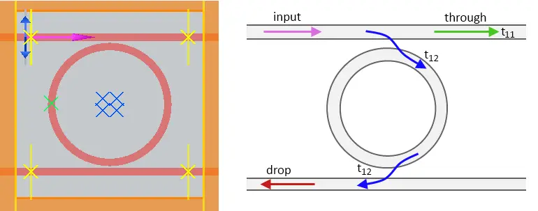
Here we use a simple ring resonator to demonstrate the varFDTD solver in Lumerical MODE.
Figure 2: a four-port ring resonator
Lumerical MODE collapses the 3D geometry into a 2D set of effective materials automatically. The effective materials produced are also dispersive. Note that the dispersion comes both from the properties of the original materials and from the geometry of the slab waveguide. The resulting materials are then fitted, using Ansys’s own Multi-Coefficient Materials model, into a form suitable for simulation by the FDTD algorithm.
Figure 3: (left) waveguide dispersion is visible in the mode profile of the vertical slab, shown as a function of the vertical dimension z and wavelength; (right) the effective material produced contains both the waveguide dispersion due to the slab waveguide geometry and the material dispersion of silicon
Once the effectively 2D materials have been produced, the 2D FDTD simulation can proceed using Ansys’s optimised compute accelerator, which allows parallel computation on multi-core processors and multi-node high performance computing systems.
Figure 4: a 2D FDTD simulation using effective 2D materials gives the broadband response from a single simulation in the time domain
The built-in eigenmode expansion monitor gives high-resolution, accurate broadband transmission data for any waveguide mode from a single simulation. Figure 5 shows the signal transmitted into the fundamental mode at the through-port position. As Table 1 shows, varFDTD agrees very closely with the 3D FDTD result and is 100 times faster. Figure 5 also compares 2D FDTD (where the index is simply the effective index of the vertical slab mode) against 3D FDTD, and the agreement there is poor. In particular, bandwidth and FSR (free spectral range), the key quantities usually extracted from such a simulation, are computed very accurately by varFDTD but not by standard 2D FDTD. To make varFDTD, 2D FDTD and 3D FDTD easier to compare, both plots in Figure 5 shift the central peak of the varFDTD and 2D FDTD transmission spectra to coincide with the 3D FDTD result. In practice this precise peak alignment can be achieved by thermal tuning.
Figure 5: (left) transmission into the fundamental mode at the through port from the varFDTD and 3D FDTD simulations; (right) results from the standard two-dimensional FDTD approximation and from three-dimensional FDTD
Simulation type
Memory
Run time on a 2010-model Intel Core i7 machine
2D FDTD
15MB
about 12 seconds
2.5D FDTD
18MB
about 15 seconds
3D FDTD
338MB
about 150 seconds
Table 1: summary of the simulation time and memory required for the ring resonator example. In this case 2D FDTD and varFDTD run about 100 times faster than 3D FDTD
Given the accuracy and speed the varFDTD solver delivers, Lumerical MODE can move ring resonator optimisation forward considerably. Because simulating ring resonators and other silicon photonic devices normally requires a larger simulation region and a longer simulation time, the varFDTD solver plays a very important part in optimising designs at this level of complexity.
Application examples: broadband analysis of planar tapers, AWGs and nonlinear waveguides
Planar tapers:
The varFDTD solver makes it straightforward to determine accurately the broadband transmission into the several modes a wide taper supports. Collapsing the vertical structure into an effective slab works perfectly over a wide region such as a taper, so no approximation is made to light propagation within the waveguide slab and this variational FDTD treatment gives results very close to 3D FDTD .
Figure 6: varFDTD simulation of an SOI waveguide taper. The taper shape is parameterised as w(x)=[α(L-x) ]^m+w_2 and optimised using the optimisation framework built into Lumerical MODE.Figure 7: transmission into the first five even TE modes of waveguide 2 at a wavelength of 1550 nm.
Arrayed waveguide gratings (AWG):
AWGs are essential devices for dense wavelength division multiplexing in optical networks. Their size and complexity, and their sensitivity to phase error, can make AWGs difficult for many propagation methods to compute. With the varFDTD solver in Lumerical MODE, accurate broadband results can be obtained from a single simulation.
Figure 8: wavelength-dependent demultiplexing visible in the output star coupler of an AWG simulated with the varFDTD solver. All of these results come from a single simulation in the time domain.
Nonlinear waveguides:
Simulating nonlinear effects in a waveguide often requires long simulation times and long propagation distances. Combining the varFDTD solver with the flexible material plugins provided by Lumerical MODE makes it possible to simulate long-distance wave propagation efficiently while capturing the interaction between linear and nonlinear effects accurately.Flexible material plugins is built on an open framework, and end users can develop models tailored to their own needs as dynamic link library plugins written in native C, C++ or FORTRAN. Used together with the multi-coefficient material model, these plugins can simulate complex nonlinear materials such as the one in Figure 9.
Figure 9: 2.5D FDTD simulation of four-wave mixing (FWM) in a nonlinear ring resonator. (left) through and drop outputs; (right) spectrum showing the pump, signal and converted light
Summary: varFDTD optimises virtual prototyping of large integrated optical components
The varFDTD solver in Lumerical MODE is a general-purpose solver for simulating broadband, omnidirectional light propagation in waveguide components. For planar geometries where coupling between different slab modes is negligible, varFDTD achieves results comparable to 3D FDTD with only the simulation time and memory of 2D FDTD. Combined with the eigenmode solver and the bidirectional eigenmode expansion (EME) solver, Lumerical MODE becomes an excellent tool for virtual prototyping of large integrated optical components, reducing the need for expensive and time-consuming fabricated prototypes.
References
[1] Manfred Hammer and Olena V. Ivanova, MESA Institute for Nanotechnology, University of Twente, Enschede, The Netherlands, “Effective index approximation of photonic crystal slabs: a 2-to-1-D assessment”, Optical and Quantum Electronics, Volume 41, Number 4, 267-283, DOI: 10.1007/s11082-009-9349-3. [2] Allan W. Snyder and John D. Love, Optical Waveguide Theory. Chapman & Hall, London, England, 1983.
We may request cookies to be set on your device. We use cookies to let us know when you visit our websites, how you interact with us, to enrich your user experience, and to customize your relationship with our website.
Click on the different category headings to find out more. You can also change some of your preferences. Note that blocking some types of cookies may impact your experience on our websites and the services we are able to offer.
Essential Website Cookies
These cookies are strictly necessary to provide you with services available through our website and to use some of its features.
Because these cookies are strictly necessary to deliver the website, refusing them will have impact how our site functions. You always can block or delete cookies by changing your browser settings and force blocking all cookies on this website. But this will always prompt you to accept/refuse cookies when revisiting our site.
We fully respect if you want to refuse cookies but to avoid asking you again and again kindly allow us to store a cookie for that. You are free to opt out any time or opt in for other cookies to get a better experience. If you refuse cookies we will remove all set cookies in our domain.
We provide you with a list of stored cookies on your computer in our domain so you can check what we stored. Due to security reasons we are not able to show or modify cookies from other domains. You can check these in your browser security settings.
Google Analytics Cookies
These cookies collect information that is used either in aggregate form to help us understand how our website is being used or how effective our marketing campaigns are, or to help us customize our website and application for you in order to enhance your experience.
If you do not want that we track your visit to our site you can disable tracking in your browser here:
Other external services
We also use different external services like Google Webfonts, Google Maps, and external Video providers. Since these providers may collect personal data like your IP address we allow you to block them here. Please be aware that this might heavily reduce the functionality and appearance of our site. Changes will take effect once you reload the page.
Google Webfont Settings:
Google Map Settings:
Google reCaptcha Settings:
Vimeo and Youtube video embeds:
Other cookies
The following cookies are also needed - You can choose if you want to allow them:
Privacy Policy
You can read about our cookies and privacy settings in detail on our Privacy Policy Page.