
Home/Analysis Technologies/Waveguide and propagation analysis/EME

Analysis Technologies | Waveguide and Propagation Analysis

EME (Eigenmode Expansion)

A frequency-domain method that divides the structure into cells along the propagation direction, takes the modes of each cross-section as a basis, and connects scattering matrices to obtain bidirectional propagation through the whole device. It suits evaluating long devices and sweeping their length.

Formulation

Bidirectional eigenmode expansion in the frequency domain

Problem solved

Mode matching at cell boundaries, connected by scattering matrices

Supporting products

Lumerical MODE
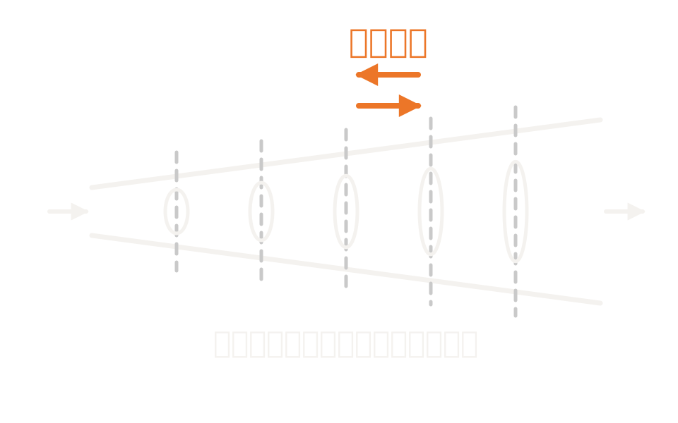
Diagram showing a structure divided into cells along the propagation direction, with the modes of each cross-section obtained and connected by scattering matrices

What the method is

Cross-sectional modes as a basis, connected along the length

This method solves Maxwell’s equations in the frequency domain. The structure is divided into several cells along the propagation direction, and modes are obtained at the boundaries between adjacent cells. At each boundary the tangential components of the electric and magnetic fields are matched, producing a scattering matrix for each section.

Propagating the section scattering matrices in both directions and connecting them gives the scattering matrix of the whole device. Because it is fully vectorial and bidirectional, reflection and backward-travelling components are included in the result.

Once the expensive stage of computing the modes is done, the propagation distance of each section can be changed at will without redoing it. That property is why a length sweep costs almost nothing extra.

How it works

Obtain modes per cell, connect with scattering matrices

Within each cell the structure is taken as uniform along the propagation direction, and modes are computed at the cell’s central cross-section. Within a cell each mode advances in phase analytically, so no grid is needed along the propagation direction. That is why the grid dispersion that appears over long regions in a time-domain solver does not arise.

The number of modes used as a basis is finite. That basis is really infinite-dimensional, so any finite set chosen is necessarily incomplete. The error shrinks as the number of modes grows, which makes a mode-count convergence check an obligatory step. For sections whose shape changes continuously, a subcell method (CVCS) is provided to avoid a staircase approximation.

Cell divisionThe structure is divided into cells along the propagation direction, and modes are obtained at the central cross-section of each. Cell groups let you vary how coarsely each section is divided.
Mode matchingThe tangential components of the electric and magnetic fields are matched at cell boundaries, producing an interface scattering matrix. Because the basis is finite, the interface scattering matrix does not necessarily conserve energy. How conservation is handled is a setting.
Bidirectional connectionThe section scattering matrices are propagated in both directions and connected to give the scattering matrix of the whole device. Reflection and backward propagation are included.
Convergence controlAccuracy is set by the number of modes, the number of cells and the cross-sectional mesh. A mode convergence sweep can reuse modes already computed for the comparison.

Strengths of this method

Why this method is chosen

Length sweeps are cheap

Changing the length of a section changes neither the modes nor the interface scattering matrices. Only the phase factor within the section changes, so only the connection of the scattering matrices has to be recomputed. In one spot size converter example, evaluating 101 taper lengths took 3 minutes, while evaluating 11 lengths of the same device with a three-dimensional time-domain solver took 6 hours, and the two sets of results agree well.

Scaling with propagation distance

The method scales extremely well with propagation distance and suits the analysis of long structures. With time-domain methods, run time grows substantially as a device gets longer.

No grid dispersion

Because propagation is handled analytically, the grid dispersion that becomes a problem in time-domain calculations over large regions does not arise. It is fully vectorial and bidirectional, and reflection is included in the result.

Where it fits

Where it fits, and where it does not

Where it is a good fit

→ when you are looking for the optimum length of a taper or spot size converter

→ when you are settling the length of the central section of an MMI coupler

→ when you need transmission and reflection of a long device as S-parameters

→ when you want the coupling length of a directional coupler from a mode basis

→ when you need S-parameters to pass to circuit simulation

Where another method is the better fit

When you want a broadband response in one go: this is a frequency-domain method, and wavelength dependence comes from a sweep. If you want a wide-band response at once, a 2.5D time-domain solver suits better.

Systems dominated by radiation or substrate leakage: where radiation or leakage into the substrate is present, those modes have to be included in the basis and the analysis becomes complicated. For arrangements such as edge couplers that involve substrate leakage, the mode search range ends up being specified by hand.

Structures with no assumable propagation axis: structures where light circulates in-plane with no defined propagation axis, such as ring resonators and photonic crystal cavities, are a poor fit. A method that assumes no propagation axis suits better.

Final accuracy confirmation: the slower three-dimensional time-domain calculation belongs on the side that verifies this method’s results. In practice it pays to separate design exploration from final confirmation.

Applications

Typical applications

Tapers and spot size converters

Sweep the taper length to find where transmission saturates, and settle the device length required.

MMI couplers

Sweep the length of the central section to find the length at which the splitting ratio matches the design value.

Edge couplers

Sweep the length of the taper joining fiber and chip, and find the optimum including leakage into the substrate.

S-parameter extraction for a circuit model

Obtain S-parameters from a wavelength sweep and use them as an element in circuit simulation.

Inputs and outputs

What you provide, and what you get

INPUT

Structure and materials The three-dimensional geometry of the sections along the propagation direction, with the material of each region
Cell settings Number of cell groups, the range and cell count of each group, and the subcell method (none or CVCS)
Number of modes A mode count common to all cells, or a mode count specified per section
Ports The position and extent of the ports at each end, the incident mode, and the number of trial modes
Cross-sectional mesh and boundary conditions The cross-sectional mesh step, and boundary conditions such as PML
Sweep conditions The range and number of points for a length sweep, the range for a wavelength sweep, and the settings for a mode convergence sweep

OUTPUT

Scattering matrix S-parameters between ports, and the transmission and reflection that follow from them
Field distribution The field distribution inside the device, reconstructed by monitors
Port mode information The effective index and field profile of the port modes, and the port mode power
Sweep results Scattering matrices against a length sweep, a wavelength sweep or a mode convergence sweep. Group delay is also available
Error diagnostics Energy conservation violation, mode basis expansion error, field discontinuity, and the forward and backward components of each mode

How it works

How it works in practice

01

Place the structure and ports

Build the three-dimensional geometry of the device, place ports at each end of the analysis region, and choose the incident mode.

02

Divide into cell groups

Divide into sections by function, such as input, transition and output, and where the shape changes continuously either increase the cell count or use the subcell method.

03

Decide the number of modes

Vary the mode count in a mode convergence sweep, compare the scattering matrices, and choose the count at which the result stops moving. Check the cell count and cross-sectional mesh the same way.

04

Sweep the length and evaluate

Sweep the section length to evaluate transmission, and where needed run a wavelength sweep for the wavelength dependence of the S-parameters.

Always check the error diagnostics. They show energy conservation violation, field discontinuity and mode basis expansion error. Where the expansion error is large, increase the mode count on both sides of that boundary. Once the design is narrowed down, verify the result with a three-dimensional time-domain calculation.

Comparison with related methods

Choosing between related analysis methods

Method Relationship Main targets When to use which
EME (this method) This method Long devices whose shape changes along the propagation direction Takes the cross-sectional modes of each cell as a basis and connects scattering matrices bidirectionally to obtain propagation through the whole device. Length sweeps are cheap.
FDE Upstream Modes of a fixed cross-section Solves the cross-sectional eigenvalue problem to obtain the modes. The modes this method uses as a basis are computed with that same solver.
varFDTD Alternative Wide planar structures, and broadband A two-dimensional time-domain calculation with the vertical direction collapsed. It suits getting a broadband result in one go, and structures with no definable propagation axis.
FDTD Complementary Final accuracy confirmation Discretizes the analysis region as a volume. It is heavier, but suits verifying this method’s results.

View all analysis technologies →

Supporting products

Products that provide this method

A commercial software environment for waveguide and optical coupling analysis. Alongside eigenmode expansion, finite-difference eigenmode analysis and 2.5D variational FDTD solvers sit in the same environment, so you can go from cross-sectional modes to whole-device propagation without leaving it. See here for licensing, system requirements and deployment.

Lumerical MODE

View the product page →

FAQ

Frequently asked questions

How many modes do I need?It varies with the structure, and there is no generally applicable number. Use a mode convergence sweep to confirm the count at which the result stops moving. In a straight taper example, results settle at around 20.
Do I have to recompute every time I change the length?No. The modes and interface scattering matrices do not depend on length, so changing the length only requires recomputing the connection of the scattering matrices. That is why length sweeps are cheap with this method.
Which is more accurate, this or a time-domain method?Both are rigorous formulations of Maxwell’s equations and become exact in the limit of fine discretization. This method’s error comes from the mode basis being finite; a time-domain method’s error comes from the grid and time step. In practice the two agree well, and a three-dimensional time-domain calculation is used for final confirmation.
What should I look at in the error diagnostics?The main indicators are energy conservation violation, discontinuity in the tangential field components, and mode basis expansion error. At a boundary where the expansion error is large, increase the mode count on both sides. For structures with sharp discontinuities, a trade-off between field continuity and energy conservation is sometimes necessary.

References

Last updated

2026-08-19

Technical review

LightBridge Technical Support

Sources consulted

Ansys Optics: MODE – EigenMode Expansion (EME) solver introductionAnsys Optics: EME solver – Simulation objectAnsys Optics: EME solver cells – Simulation objectAnsys Optics: EME solver ports – Simulation objectAnsys Optics: EME Solver analysis window overviewAnsys Optics: Understanding EME error diagnosticsAnsys Optics: Convergence testing process for EME simulationsAnsys Optics: Spot size converterAnsys Optics: Linear waveguide taperAnsys Optics: Multi-Mode Interference (MMI) Coupler

We can advise on propagation analysis of long waveguide devices

Tell us the make-up of the device and the dimensions you need to settle, and we will propose the method and product that suit.