Home/Analysis Technologies/Waveguide and propagation analysis/FDE

Analysis Technologies | Waveguide and Propagation Analysis

FDE (Finite-Difference Eigenmode)

A method that discretizes the cross-section of a waveguide uniform along the propagation direction by finite differences and solves Maxwell’s equations as a sparse eigenvalue problem, giving the effective index, field profile and loss of each mode.

Discretization

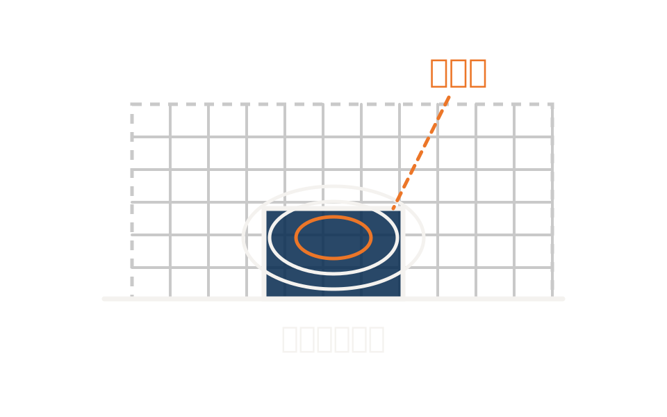
Finite-difference mesh on the cross-section

Problem solved

Two-dimensional eigenvalue problem on the cross-section

Supporting products

Lumerical MODE

Diagram showing the cross-section of a waveguide uniform along the propagation direction divided by an orthogonal grid, with the mode field distributed over it

What the method is

Obtaining the modes from a waveguide cross-section

How light travels along a waveguide is set by the discrete modes its cross-section supports. This method solves Maxwell’s equations on a mesh of the waveguide cross-section and obtains the spatial distribution and frequency dependence of the modes.

What you get is the field profile, effective index and loss for each mode. The effective index is defined from the propagation constant and the angular frequency, and for materials with a complex refractive index the imaginary part becomes propagation loss. Fields are normalized so that the peak electric field intensity is 1.

The cross-section is divided by a rectangular mesh. The default is uniform, but grading, local refinement and conformal treatment of material interfaces can also be selected. A frequency sweep capability lets you go straight on to group delay and dispersion.

How it works

Finite-difference discretization on the cross-sectional mesh, solved as a sparse eigenvalue problem

The method starts from the premise that the structure is uniform along the propagation direction. Under that premise, separating the fields into an in-plane distribution and a term whose phase advances along the propagation direction turns a three-dimensional problem into a two-dimensional one on the cross-section. Finite differences discretize that on a mesh covering the cross-section and rewrite it as a matrix eigenvalue problem whose eigenvalue is the square of the propagation constant. The resulting matrix is sparse and is solved with a sparse solver.

Mode selection is not automatic. You have to give the wavelength to solve at, the number of trial modes to return, and the effective index to search around. Take a generous number of trial modes so that a physical mode near your target is not missed. Note too that using symmetric boundaries can leave only one polarization.

AssumptionsOn the premise that the structure is uniform along the propagation direction, the fields are written as the product of an in-plane distribution and a phase term along the propagation direction.
DiscretizationThe cross-section is divided by a rectangular mesh and discretized by finite differences. Grading, local refinement and conformal treatment of material interfaces are available. There is no points-per-wavelength requirement of the kind time-domain solvers have.
FormulationMaxwell’s equations become a matrix eigenvalue problem. The eigenvalue corresponds to the square of the propagation constant, and the eigenvector is the mode field profile.
NormalizationEach mode field is normalized so that the peak electric field intensity is 1.

Strengths of this method

Why this method is chosen

Cost set by the cross-section alone

What sets the cost is the cross-sectional mesh, not the length of the device or any time stepping. One eigenvalue solve at one frequency returns all the supported modes at once.

Built-in frequency sweep

A sweep capability is built in, giving group index, group velocity, group delay and dispersion as functions of wavelength. You can also track a particular mode through the sweep.

Bent waveguides and leakage loss

Modes of a bent waveguide can be solved by specifying the bend radius, orientation and reference point. With PML boundaries, the fraction radiated away by the bend can be evaluated as loss.

Where it fits

Where it fits, and where it does not

Where it is a good fit

→ when you need effective index, group index, dispersion and loss from the cross-section of a waveguide uniform along the propagation direction

→ when you want to sweep wavelength and obtain the wavelength dependence of group delay and dispersion together

→ when you want to evaluate the modes of a bent waveguide and the radiation loss from the bend

→ when you want to estimate the coupling fraction at a junction from the overlap of two modes

→ when you want to extract waveguide element parameters to pass to circuit simulation

Where another method is the better fit

Devices whose shape changes along the propagation direction: what this method returns is the modes supported by a fixed cross-section. If you need transmission or reflection of a device whose shape changes along the propagation direction, such as a taper or an MMI, you need a method that uses those modes as a basis and connects along the length.

Structures propagating widely in-plane: it does not suit structures such as ring resonators or AWGs where light circulates in-plane with no defined propagation axis. A method that collapses the vertical direction and solves in-plane in the time domain suits better.

Three-dimensional scattering and radiation: if you need whole-device scattering, far fields or S-parameters, you need a method that discretizes the analysis region as a volume.

If you expect modes to be selected for you: the mode you want is not selected automatically. You have to give the number of trial modes and the effective index to search around, and depending on the symmetric boundaries you choose, only one polarization may remain.

Applications

Typical applications

Characterizing silicon photonics waveguides

Obtain the mode profile, effective index, loss, polarization fraction and effective area of an SOI waveguide.

Dispersion design

Sweep wavelength to obtain group index and dispersion, as the basis for settling waveguide dimensions.

Estimating bend loss

Solve the modes at a specified bend radius and evaluate propagation loss separately from the overlap mismatch at the junction with the straight section.

Parameter extraction for a circuit model

Obtain the wavelength dependence of effective index and group index and pass them to the waveguide element in circuit simulation.

Inputs and outputs

What you provide, and what you get

INPUT

Cross-sectional geometry The cross-section of a waveguide that can be taken as uniform along the propagation direction, with the material of each region
Material Refractive index data. Anisotropic materials and complex indices are supported
Analysis conditions Wavelength or frequency, the number of trial modes, and the effective index value or range to search
Mesh Number of mesh cells or maximum mesh step, grading factor, minimum mesh step, local refinement
Boundary conditions PML, metal (PEC), PMC, periodic, symmetric and antisymmetric
Bend Bend radius, bend orientation, bend reference point

OUTPUT

Effective index and loss Effective index per mode, and propagation loss (dB/m) for materials with a complex index
Mode profile Each component of the electric and magnetic fields on the cross-section
Mode properties TE polarization fraction, guided TE/TM fraction, effective area
Frequency sweep results Wavelength dependence of effective index, loss, group index, group velocity, group delay, dispersion and propagation constant
Overlap between modes The overlap of two modes and the coupling fraction that follows from it

How it works

How it works in practice

01

Define the cross-section and materials

Build a cross-section that can be taken as uniform along the propagation direction and assign materials such as core, cladding and substrate.

02

Settle the analysis region, mesh and boundary conditions

Take a region wide enough that the mode tail does not reach the boundary, and set the mesh step and boundary conditions. Use PML if radiation is to be included.

03

Solve the modes and select

Give the wavelength, the number of trial modes and the effective index to search around, run the calculation, and pick the mode you want from the mode list.

04

Sweep wavelength to obtain the characteristics

Run a frequency sweep while tracking the mode you selected, and obtain the wavelength dependence of effective index, group index, dispersion and loss.

Refine the mesh and confirm that effective index and loss stop moving. If the analysis region is too narrow, the mode tail reflects at the boundary and the result changes. To obtain dispersion accurately, use the setting that computes at additional frequency points.

Comparison with related methods

Choosing between related analysis methods

Method Relationship Main targets When to use which
FDE (this method) This method Cross-section of a waveguide uniform along the propagation direction Discretizes the cross-sectional mesh by finite differences and solves an eigenvalue problem for mode effective index and field profile. A frequency sweep gives dispersion as well.
FEEM Alternative Cross-sections including curved surfaces Solves the same cross-sectional eigenvalue problem with triangular finite elements. The mesh can follow material interfaces, and normalization is based on the power each mode carries.
EME Downstream Long devices whose shape changes along the propagation direction Takes the modes of each cross-section as a basis and connects scattering matrices to obtain propagation through the whole device. That mode calculation uses this method’s solver.
varFDTD Alternative Wide planar structures Collapses the vertical direction into an effective index and handles in-plane propagation with a two-dimensional time-domain calculation.
FDTD Complementary Three-dimensional structures at wavelength scale Discretizes the analysis region as a volume and gives spectra, far fields and S-parameters.

View all analysis technologies →

Supporting products

Products that provide this method

A commercial software environment for waveguide and optical coupling analysis. Alongside finite-difference eigenmode analysis, eigenmode expansion and 2.5D variational FDTD solvers sit in the same environment, so you can go from cross-sectional modes to whole-device propagation without leaving it. See here for licensing, system requirements and deployment.

Lumerical MODE

View the product page →

FAQ

Frequently asked questions

How does this differ from finite-element mode analysis?The quantities obtained are of the same kind, but the discretization and normalization differ. This method divides the cross-section by finite differences on a rectangular mesh, and fields are normalized so that the peak electric field intensity is 1. A finite-element solver can align triangular elements with material interfaces. The frequency sweep capability is on this side.
Are modes found automatically?No. You have to give the number of trial modes to return and the effective index to search around. Take a generous number of trial modes so that a physical mode is not missed. Using symmetric boundaries can leave only one polarization.
Can it give group index and dispersion?There is a frequency sweep capability, and it can output effective index, loss, group index, group velocity, group delay, dispersion and propagation constant as functions of wavelength. There are settings for tracking a particular mode and for computing dispersion in detail.
Can it evaluate bend loss?Modes of a bent waveguide can be solved by specifying the bend radius, orientation and reference point. Radiation from the bend is absorbed at PML boundaries and evaluated as loss. At the junction between curved and straight sections, the loss from mode overlap mismatch is evaluated separately.

References

Last updated

2026-08-19

Technical review

LightBridge Technical Support

Sources consulted

Ansys Optics: MODE – Finite Difference Eigenmode (FDE) solver introductionAnsys Optics: FDE solver – Simulation objectAnsys Optics: FDE solver analysis – Modal Analysis TabAnsys Optics: FDE solver analysis – Mode List and DeckAnsys Optics: Frequency Analysis – Modal Analysis TabAnsys Optics: Solving bent waveguides in FDE and FEEMAnsys Optics: Tips for finding modes in FDE and the mode sourceAnsys Optics: MODE product reference manual

We can advise on waveguide mode analysis

Tell us the make-up of the cross-section and the characteristics you want to evaluate, and we will propose the method and product that suit.