Home/Analysis Technologies/Performance evaluation/Image Quality Analysis

Analysis Technologies | Performance Evaluation

Image Quality Analysis

A grouping of analysis capabilities for evaluating the performance of an imaging system. There are metrics based on geometric rays and metrics based on diffraction, used according to the aberration level, the purpose of the evaluation and the computation conditions.

Where it sits

A grouping of analysis capabilities for evaluating imaging performance

Two foundations

Quantities based on geometric rays, and on diffraction

Supporting products

Ansys Zemax OpticStudio

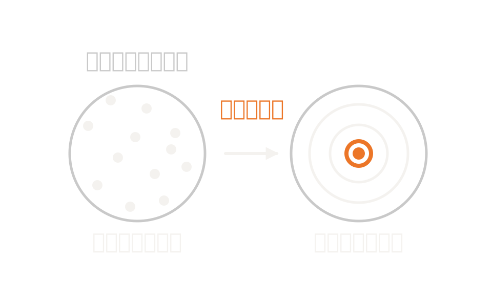
Diagram showing geometric metrics working where aberrations are large and diffraction metrics working near the diffraction limit

What the method is

Decide which metric to look at first

In OpticStudio, evaluation of imaging performance is gathered in the Image Quality group of the Analyze tab. That group holds the analyses used for designing imaging and afocal systems: ray trace data, aberration data, wavefront, point spread function and so on. It is the name of a group of capabilities, not of a single one.

The group has eight subcategories: rays and spots, aberrations, wavefront, point spread function, MTF, RMS, encircled energy and extended scene analysis. This page deals mainly with those that have no page of their own, pointing to the respective pages for contrast at each spatial frequency and for evaluation of the wavefront itself.

The metrics divide broadly into those based on geometric rays and those based on diffraction. The former express where the rays land, the latter the intensity distribution as a wave. Which to use is decided by how close the system is to the diffraction limit.

How it works

Choose between geometric and diffraction-based metrics according to aberration level, purpose and computation conditions

It is not the size of the aberrations alone that decides. Three things do: the aberration level, the purpose of the evaluation, and the computation conditions. In systems with large aberrations, where the rays land more or less decides the performance, so spot diagrams, ray aberration plots, geometric MTF and geometric encircled energy work well. As a system approaches the diffraction limit, ray spread no longer describes performance, and you move to diffraction-based metrics such as the point spread function and the Strehl ratio. Purpose matters too: whether you are asking about contrast, about the fraction of energy, or about how it actually looks changes the metric you choose. Computation conditions matter as well: depending on f-number, image plane tilt, exit pupil distortion and sampling density, the diffraction calculation itself may not hold.

There are several concrete guides on aberration level. On a spot diagram, if all the rays fall well inside the Airy disc, the system can be taken as diffraction limited. For diffraction-based MTF, switch to geometric MTF once the wavefront error exceeds about 10 waves. Image simulation switches automatically from a diffraction point spread to a geometric one at 20 times the diffraction limit. The Strehl ratio approximation from Zernike coefficients is only usable for monochromatic light and where the Strehl ratio is above about 0.10. These are guides: judge them together with the purpose of the evaluation and the computation conditions.

Rays and spotsTrace a bundle of rays and look at the distribution at the image plane. The geometric spot radius is the distance to the furthest ray from the reference point; the RMS spot radius is the root mean square of the distances of the rays from it. The Airy disc can be overlaid.
Point spread functionThe intensity distribution arising from a point source. There is an FFT calculation and one that integrates the Huygens wavefront directly. The former carries premises such as the image plane being in the far field; the latter has fewer premises but takes longer.
Encircled energyShows how much of the total energy falls within a given distance from the chief ray or the image centroid. Circular, square and one-directional shapes can be selected.
Extended scene evaluationImage simulation convolves an array of point spread functions with a bitmap to form an image. Diffraction, aberration, distortion, relative illumination, image orientation and polarization are taken into account.

Strengths of this method

Why this method is chosen

A metric matched to the question

Blur size, how energy gathers, the shape of the point image, how it actually looks: there is a metric for each thing you might want to know. The same design can be checked from several angles.

There are clues for choosing the metric

There are concrete guides: falling within the Airy disc, wavefront error of about 10 waves, 20 times the diffraction limit, a Strehl ratio of about 0.10. Considered together with the purpose and the computation conditions, the choice of metric need not rest on instinct.

Field, wavelength and focus can be scanned

RMS wavefront error, RMS spot radius and Strehl ratio can be plotted as functions of field, wavelength and defocus. The whole field can also be seen as a two-dimensional map.

Where it fits

Where it fits, and where it does not

Where it is a good fit

→ when you want to settle first which metric should describe performance

→ when you want to compare blur size quickly while aberrations are still large

→ when you need to know how energy gathers relative to a detector pixel or an aperture

→ when you want to follow performance against field, wavelength and defocus with a single number

→ when you want to show how a real scene would be captured

Where another method is the better fit

Contrast at each spatial frequency: if the resolution specification is expressed as contrast against spatial frequency, go to the modulation transfer function page. It covers the three calculation methods and the premises of each.

The shape of the wavefront itself, and the breakdown of aberrations: if you want to know what to correct and by how much, go to the wavefront analysis page. It covers departure from the reference sphere, Zernike coefficients and Seidel coefficients.

Propagation of a coherent beam: laser beam propagation, fiber coupling and the diffraction rings arising at an aperture edge cannot be expressed by imaging performance metrics. Move to physical optics propagation, which carries the field itself from surface to surface.

Evaluating unintended light: where light that does not contribute to the image is the problem, such as ghosting or internal scattering, stray light analysis takes over.

Applications

Typical applications

Evaluating cameras and imaging optics

Evaluate blur size, how energy gathers and appearance together across the whole field.

Designing to the detector pixel

Use encircled energy and make the light falling within the pixel size the design criterion.

Comparison while aberrations are large

Early in design, compare several candidates quickly with spot radius and ray aberration plots.

Showing how it looks

Produce a photographic-looking image and share what will actually be seen, rather than specification figures.

Inputs and outputs

What you provide, and what you get

INPUT

Design data Surface shapes and materials, and the stop setting
Field and wavelength The field points and wavelengths defined. Most analyses return results per field and wavelength
Sampling density The density of the ray grid across the pupil. In diffraction calculations it governs whether the result is correct
Evaluation surface The image plane, or an intermediate surface
Polarization The setting for whether polarization is taken into account

OUTPUT

Spot size Geometric spot radius, RMS spot radius, Airy disc radius
Point spread The intensity distribution for a point source, and the Strehl ratio
Encircled energy The fraction of energy enclosed against distance from the reference point
RMS scans RMS wavefront error, RMS spot radius and Strehl ratio against field, wavelength and defocus
Appearance Image simulation results from a bitmap input, and the efficiency of geometric image analysis

How it works

How it works in practice

01

Settle the stop, field and wavelengths

Evaluation presumes these three. Decide first at which field points and wavelengths the specification is stated.

02

Look at the whole with geometric metrics

Get a sense of the size and type of the aberrations from spot diagrams and ray aberration plots. Judge how close you are to the diffraction limit by comparison with the Airy disc.

03

Switch to diffraction metrics

For systems near the diffraction limit, move to the point spread function and diffraction-based encircled energy. Refine the sampling and confirm the result stops moving.

04

Close with the metric that matches the specification

A contrast specification calls for the modulation transfer function, an energy specification for encircled energy, an appearance specification for image simulation: conclude with the metric whose form matches the specification.

Diffraction calculations depend on sampling density. A warning that the sampling is insufficient may appear. Refine it in stages and confirm the point at which the result stops moving. Note also that spot diagrams do not draw vignetted rays, nor use them in the RMS or geometric radius calculation.

Relationship to related methods

Division of roles and coupling with related analysis methods

Method Relationship Main targets When to use which
Image quality analysis (this method) This method The overall picture of imaging performance Covers spot, point spread, encircled energy, RMS scans and extended scene evaluation together. Deciding when to switch between geometric and diffraction metrics is part of it.
MTF Complementary Contrast at each spatial frequency The metric that turns a resolution specification into a number. There are three calculation methods, each with different premises.
Wavefront Analysis Complementary The breakdown and size of the aberrations Measures departure from the reference sphere and decomposes it into orthogonal polynomials. The metric for knowing what to correct.
Physical Optics Propagation Alternative Propagation of a coherent beam Carries a complex amplitude field from surface to surface. Fiber coupling and beam waist evaluation belong here, not to imaging performance metrics.

View all analysis technologies →

Supporting products

Products that provide this method

Commercial software used for the design and analysis of imaging, illumination and laser systems. It provides imaging performance evaluation based on both geometry and diffraction, and continues through optimization and tolerance analysis in the same environment. See here for licensing, system requirements and deployment.

Ansys Zemax OpticStudio

View the product page →

FAQ

Frequently asked questions

Is there a single capability called image quality analysis?No. It is the name of the Image Quality group on OpticStudio’s Analyze tab, where the analyses used for designing imaging and afocal systems are gathered. What this page covers is how to choose between the metrics in that group.
Where do I switch between geometric and diffraction metrics?There are concrete guides on aberration level. If all the rays fall well inside the Airy disc, the system can be taken as diffraction limited. Once the wavefront error exceeds about 10 waves, switch from diffraction-based MTF to geometric MTF. Image simulation switches automatically at 20 times the diffraction limit. Aberration level alone does not decide it, though: judge together with the purpose and with computation conditions such as f-number, image plane tilt and sampling density.
Is a spot diagram enough?While aberrations are large, yes. As you approach the diffraction limit, ray spread stops representing the real intensity distribution. Judge whether you have entered that regime by comparison with the Airy disc, then move to the point spread function and encircled energy.
When can I use the Strehl ratio?The rigorous one is computed from a point spread obtained by direct integration of the Huygens wavefront. The approximation from Zernike coefficients is only usable for monochromatic light and where the Strehl ratio is above about 0.10. In field scans too, Strehl ratio can only be selected for monochromatic light.

References

Last updated

2026-08-19

Technical review

LightBridge Technical Support

Sources consulted

Ansys Zemax OpticStudio User Guide: The Analyze Tab (sequential ui mode)Ansys Zemax OpticStudio User Guide: Image Quality GroupAnsys Zemax OpticStudio User Guide: Standard Spot DiagramAnsys Zemax OpticStudio User Guide: FFT PSFAnsys Zemax OpticStudio User Guide: Huygens PSFAnsys Zemax OpticStudio User Guide: Diffraction (enclosed energy)Ansys Zemax OpticStudio User Guide: Image SimulationAnsys Zemax OpticStudio User Guide: RMS vs. FieldAnsys Optics: What is a Point Spread Function?

We can advise on which metric should describe imaging performance

Tell us how the optical system is put together and the specification you need to hold, and we will propose how to evaluate it.