Home/Analysis Technologies/Performance evaluation/Wavefront Analysis

Analysis Technologies | Performance Evaluation

Wavefront Analysis

An evaluation capability that measures the departure of the wavefront from a reference sphere at the exit pupil and expresses it as a distribution across the pupil with PV and RMS values. Where a breakdown of the aberrations is needed, it decomposes into Zernike polynomials.

Quantity handled

Departure from the reference sphere at the exit pupil

Units

Quantities in units of the wavelength

Supporting products

Ansys Zemax OpticStudio

Diagram showing the wavefront departing from the reference sphere at the exit pupil, and that departure decomposed into polynomial components where needed

What the method is

Measuring aberration as departure from a reference sphere

Optical path difference is defined as the difference between the optical path length of a given ray and that of the chief ray. OpticStudio expresses that quantity in units of each wavelength and computes it as reduced to the path difference at the system’s exit pupil. The wavefront map displays that error across the whole pupil.

The reference is by default the reference sphere for the wavelength in use. Switching to the reference sphere of the primary wavelength makes the lateral shift per wavelength appear as error. There is also a setting to display with the shape of the exit pupil reflected; turning it off displays in the circular coordinates of the entrance pupil.

The basis of the evaluation is the wavefront error on the pupil itself. In many situations the wavefront map, PV and RMS values are enough to reach a judgment. When a breakdown of the aberrations is needed, the distribution across the pupil is decomposed into a set of orthogonal polynomials. That decomposition also gives the variance, the Strehl ratio and the fitting residual. The residual is what tells you whether the decomposition is sufficient.

How it works

Evaluate the wavefront error on the pupil, and decompose into Zernike polynomials where needed

Decomposition is not an obligatory step in wavefront analysis. First look at the shape across the pupil in the wavefront map and get the size from the PV and RMS values. Move on to Zernike polynomials when you want to treat which aberration contributes how much as an allocation. OpticStudio has three sets. The standard set is an orthonormal system based on Noll’s notation, in which the magnitude of each coefficient corresponds directly to that term’s RMS contribution, and up to 231 terms are supported. The fringe set is not orthonormal, is normalized to unit magnitude at the pupil edge, and has up to 37 terms. The annular set adds Mahajan’s extension to annular pupils to Noll’s notation and is used with an obscuration ratio specified. At an obscuration ratio of 0, the annular set coincides with the standard set.

The premise of the decomposition is that the rays are uniformly arranged on normalized pupil coordinates. If the rays are not uniformly sampled at the surface being evaluated, the result is not correct. For a rotationally symmetric system made only of spherical, conic, and second- or fourth-order aspheric surfaces, the classical breakdown of aberrations can be confirmed through Seidel coefficients. That calculation is valid only for systems meeting those conditions. It cannot be used for systems with coordinate breaks, diffraction gratings or non-rotationally-symmetric surfaces.

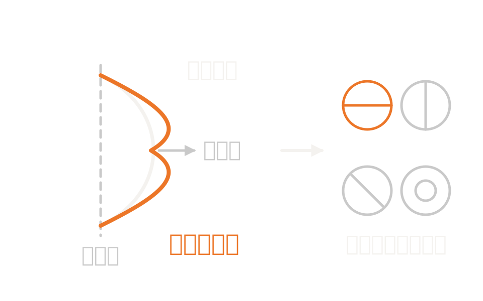
Optical path differenceThe difference in optical path length between the ray of interest and the chief ray. Expressed in units of the wavelength and computed as reduced to the difference at the exit pupil.
Choosing the referenceThe default is the reference sphere for the wavelength in use. Switching to the primary wavelength’s reference sphere makes the lateral shift per wavelength visible. Whether the exit pupil shape is reflected is also selectable.
Decomposition where neededDecompose into Zernike polynomials when a breakdown of the aberrations is needed. Choose from the standard, fringe and annular sets; in the orthonormal sets the magnitude of a coefficient corresponds to that term’s RMS contribution.
Summary figures and the validity of the decompositionPV value, RMS value, variance, Strehl ratio, and the fitting residual and maximum error are obtained.

Strengths of this method

Why this method is chosen

Aberrations broken down into numbers

Because the distribution across the pupil is decomposed into orthogonal components, which aberration contributes how much can be treated as an allocation. In the orthonormal sets, a coefficient is the RMS contribution directly.

It can be matched to the pupil shape

For an obscured annular pupil, an annular polynomial set is provided. Orthogonality is preserved on the real pupil, so the interpretation of the coefficients does not break down.

Usable for comparison with measurement

The fringe set is a convention widely used in interferometry. Coefficients can be produced in the same convention as measured data, so design and measured values can be set side by side.

Where it fits

Where it fits, and where it does not

Where it is a good fit

→ when you want to state performance as error in units of the wavelength for a system near the diffraction limit

→ when you want to see which aberration contributes how much, as an allocation of components

→ when you want to compare design and measured values in the same convention as interferometry data

→ when you want to evaluate a system with an obscured annular pupil in a convention that matches the pupil shape

→ when you want to refine a design with wavefront error as the target

Where another method is the better fit

Systems with very large aberrations: for systems where the wavefront error reaches tens of waves, describing it as a wavefront becomes unwieldy and the Strehl ratio approximation no longer holds. Return to spot radius or geometric contrast metrics.

When you want to tie it directly to a contrast specification: RMS wavefront error does not convert directly into contrast at each spatial frequency. Use the modulation transfer function for a resolution specification.

Seidel coefficients for non-rotationally-symmetric systems: the Seidel coefficient calculation is valid only for systems made of rotationally symmetric spherical, conic, and second- or fourth-order aspheric surfaces. For systems with coordinate breaks, diffraction gratings or freeform surfaces, use the wavefront map and Zernike coefficients.

Propagation of a coherent beam: what this evaluation handles is the state of the pupil aberration at one surface. What actually happens to the beam during propagation, and how much couples into a fiber, is the territory of physical optics propagation, which carries the field itself.

Applications

Typical applications

Aberration allocation in imaging systems

Separate which aberration contributes how much into components and settle the allocation between design and manufacturing.

Comparison with interferometry

Produce coefficients in the convention used in measurement and set design and measured values side by side.

Reflective systems with an annular pupil

Evaluate with annular polynomials at a specified obscuration ratio, preserving orthogonality on the real pupil shape.

Design against a wavefront error target

Put RMS wavefront error or Zernike coefficients into the operands and bring the design toward the target.

Inputs and outputs

What you provide, and what you get

INPUT

Sampling density The density of the ray grid across the pupil. The premise is that the rays are uniformly arranged on normalized pupil coordinates
Field and wavelength The field points and wavelengths evaluated
Reference settings Whether the reference sphere is that of the wavelength in use or of the primary wavelength, and whether the exit pupil shape is reflected
Polynomial settings Standard, fringe or annular, the maximum number of terms, and for the annular set the obscuration ratio
Evaluation surface The image plane, or an intermediate surface
Sub-aperture The center and radius when only part of the pupil is the subject

OUTPUT

Wavefront map The two-dimensional distribution of wavefront error across the whole pupil
Optical path difference cross-sections Curves of optical path difference along two cross-sections of the pupil
Zernike coefficients A table of coefficients according to the set and number of terms chosen, in units of the wavelength
Summary figures PV value, RMS value, variance, Strehl ratio, and the fitting residual and maximum error
Scan results Variation of Zernike coefficients across the field, and RMS wavefront error against field, wavelength and defocus

How it works

How it works in practice

01

Settle the evaluation surface and the reference

Decide whether to evaluate at the image plane or an intermediate surface, and choose which reference sphere to use.

02

Look at cross-sections, then the whole

First get the size from the optical path difference cross-sections, then look at the shape across the whole pupil in the wavefront map. Note that a cross-section shows only part of the pupil.

03

Decompose where needed

Where a breakdown is needed, choose the set that matches the pupil shape, settle the number of terms and obtain the coefficients. Check the PV value, RMS value, Strehl ratio and fitting residual. If no breakdown is needed, this stage can be skipped.

04

Scan across field and focus

Confirm the variation of the coefficients across the field, and RMS wavefront error against field, wavelength and defocus.

The premise of the decomposition is that the rays are uniformly arranged on normalized pupil coordinates. Refine the sampling and confirm the coefficients and RMS value stop moving. A large fitting residual means too few terms. Note that in a field scan of Zernike coefficients, vignetting factors are ignored. Where the phase from polarization exceeds one wave, the phase is not unwrapped, so an abrupt step appears in the wavefront map.

Relationship to related methods

Division of roles and coupling with related analysis methods

Method Relationship Main targets When to use which
Wavefront analysis (this method) This method The state of the aberration at the exit pupil Measures departure from the reference sphere and expresses it as a distribution across the pupil with PV and RMS values. Where a breakdown is needed, decomposes into Zernike polynomials.
MTF Downstream Contrast specifications The point spread follows from the wavefront data, and the contrast metric from that. It is the metric for the stage of stating a specification.
Image Quality Analysis Complementary The overall picture of performance Covers views other than pupil aberration: spot, point spread, encircled energy and appearance.
Physical Optics Propagation Alternative The field during propagation Carries a complex amplitude field from surface to surface. Beam waist movement, fiber coupling and the diffraction rings at an aperture edge belong here.

View all analysis technologies →

Supporting products

Products that provide this method

Commercial software used for the design and analysis of imaging, illumination and laser systems. Alongside aberration evaluation by wavefront map and Zernike coefficients, it provides imaging performance metrics, optimization and tolerance analysis in the same environment. See here for licensing, system requirements and deployment.

Ansys Zemax OpticStudio

View the product page →

FAQ

Frequently asked questions

How do I choose between the three Zernike sets?The standard set is an orthonormal system based on Noll’s notation, in which a coefficient’s magnitude corresponds to that term’s RMS contribution. The fringe set is not orthonormal, is normalized to unit magnitude at the pupil edge, and is the convention used in interferometry. The annular set is for obscured pupils and takes an obscuration ratio; at an obscuration ratio of 0 it coincides with the standard set.
What are the units?Optical path difference and Zernike coefficients are each expressed in units of the wavelength. The display unit of the wavefront map is not stated explicitly, so read it in wavelength units, consistent with optical path difference and Zernike coefficients.
Can Seidel coefficients always be used?No. They are valid only for systems made of rotationally symmetric spherical, conic, and second- or fourth-order aspheric surfaces. For systems with coordinate breaks, diffraction gratings or non-rotationally-symmetric surfaces, use the wavefront map and Zernike coefficients.
How does this differ from physical optics propagation?They address different things. This evaluation describes the departure from the reference sphere at the exit pupil, that is, the state of the aberration at one surface. Physical optics propagation carries the complex amplitude of a coherent beam from surface to surface and gives intensity and phase at each surface, the beam waist position, and coupling efficiency into a fiber. The former does not propagate the beam; the latter returns no decomposition into orthogonal polynomials.

References

Last updated

2026-08-19

Technical review

LightBridge Technical Support

Sources consulted

Ansys Zemax OpticStudio User Guide: WavefrontAnsys Zemax OpticStudio User Guide: Wavefront MapAnsys Zemax OpticStudio User Guide: Optical Path DifferenceAnsys Zemax OpticStudio User Guide: Zernike Standard CoefficientsAnsys Zemax OpticStudio User Guide: Zernike Fringe CoefficientsAnsys Zemax OpticStudio User Guide: Zernike Annular CoefficientsAnsys Zemax OpticStudio User Guide: Zernike Coefficients vs. FieldAnsys Zemax OpticStudio User Guide: Seidel CoefficientsAnsys Zemax OpticStudio User Guide: Physical Optics PropagationR. J. Noll, Journal of the Optical Society of America 66(3), 1976V. N. Mahajan, Journal of the Optical Society of America 71(1), 1981

We can advise on performance evaluation by wavefront error

Tell us how the optical system is put together and the aberrations you want to evaluate, and we will propose how to evaluate them.