Home/Analysis Technologies/Optical analysis/Physical Optics Propagation (POP)

Analysis Technologies | Optical Analysis

Physical Optics Propagation (POP)

A method that represents a beam as an array of complex amplitudes and propagates it from surface to surface including diffraction, carrying the phase information that ray tracing loses.

Target

Coherent beam propagation

Treatment

Propagated as an array of complex amplitudes

Supporting products

Ansys Zemax OpticStudio

Schematic showing a complex amplitude field with amplitude and phase, sampled on a finite grid and propagated from surface to surface

What the method is

Carrying a field, not rays

Ray tracing includes no interference between rays. A small beam diameter, heavy clipping at an aperture, or a need for the distribution at an intermediate surface itself: in these situations the light has to be propagated as a field with amplitude and phase.

This method carries a coherent optical field from surface to surface over the range from a specified start surface to an end surface, as an analysis within the mode that assumes surface order. The field is represented as an array of points, each holding a complex amplitude. The array size, the number of sampling points and the aspect ratio are the user’s to decide. Two algorithms are available for surface-to-surface propagation, one based on Fresnel diffraction and one on the angular spectrum, and whichever is numerically more accurate is selected automatically.

There are premises. Propagation is assumed paraxial, and as a guide a beam diverging beyond about 20 degrees half-angle falls outside that premise. The field component normal to the surface is taken as zero, so the assumption also breaks down for strongly converging or diverging beams.

How it works

Fresnel diffraction and the angular spectrum

The treatment of propagation including diffraction is organized within the framework of Fourier optics: propagation as an angular spectrum of plane waves, the Fresnel approximation, and the Fraunhofer approximation, used according to the subject and the propagation distance. The two algorithms this method holds correspond to the first two of those.

Numerically, angular spectrum propagation based on the fast Fourier transform requires the angular spectrum to be sampled on a uniform grid. Where that condition breaks, interpolation becomes necessary, and the interpolation error grows the more oblique the geometry. That is why the design of the sampling decides how far the result can be trusted.

In practice the cautions come down to sampling and the extent of the computation region. The number of sampling points is the user’s to decide, and up to 16,384 by 16,384 points can be specified from the user interface. The width of the computation region has to be taken well wider than the beam; if the region is narrow relative to the beam, the tail of the field does not fit inside it and causes wrap-around. Clipping by the system’s apertures can be handled on the field, but only on the premise that the computation region is sufficient. That is why the documented procedure is to follow the beam surface by surface and confirm there is no aliasing or other anomaly, rather than looking only at the final surface after propagating.

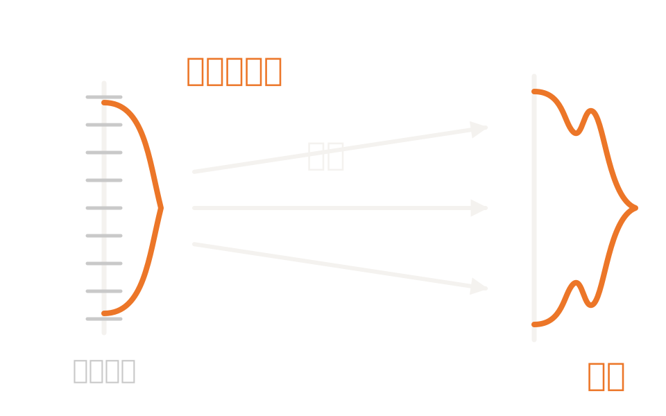
Representing the fieldThe wavefront is represented as an array of points, each holding a complex amplitude. Setting the premises amounts to deciding the array size, the number of points and the aspect ratio.
Two propagatorsSurface-to-surface propagation is by Fresnel diffraction or by the angular spectrum. Which is used is selected automatically.
Sampling and the computation regionThe number of sampling points and the width of the computation region are the user’s to decide. Take the region well wider than the beam and check surface by surface for aliasing. Angular spectrum propagation by fast Fourier transform presumes sampling on a uniform grid, and where that premise breaks, interpolation error enters.
The paraxial assumptionPropagation is assumed paraxial, and the field component normal to the surface is taken as zero. The premise breaks down for strongly converging or diverging beams.

Strengths of this method

Why this method is chosen

Phase is carried through

Because amplitude and phase propagate together, the field itself can be extracted at any intermediate surface. That is different information from a calculation that only gives the diffraction image at the image plane.

Clipping and what follows it

Because clipping by an aperture can be handled on the field, propagation including the diffraction that follows can be traced directly.

External fields can be brought in

Because it is represented as a complex amplitude on a computation grid, a field obtained from another analysis can be taken as input and passed through the optical system.

Where it fits

Where it fits, and where it does not

Where it is a good fit

→ when handling a coherent beam where diffraction decides the result

→ when you need the amplitude and phase distribution at an intermediate surface itself

→ when you want to follow the effect of clipping at an aperture

→ when you want to pass a field obtained from wavelength-scale structure analysis through a macroscopic optical system

Where another method is the better fit

Systems containing elements that assume no path: in systems containing elements where no path is assumed, the accuracy of this method is generally not guaranteed. Replace them with an equivalent model that assumes surface order.

Systems dominated by geometric aberration: where aberrations matter more than diffraction, geometric metrics such as a spot diagram are enough.

When only the diffraction image at the image plane is needed: if only the diffraction image at the image plane of an imaging system is needed, lighter diffraction calculations are provided.

Strongly diverging beams: as a guide, a beam diverging beyond 20 degrees half-angle falls outside the paraxial assumption, so rigorous electromagnetic analysis or far-field projection is more suitable.

Applications

Typical applications

Laser beam propagation

Evaluate how a Gaussian beam behaves as it passes through a real optical system.

Working with wavelength-scale structures

Pass a field obtained from metalens or grating analysis through the optical system.

Silicon Photonics

Pass fields between chip-side analysis and optical system analysis.

Metrology optics

Check the state of the beam in systems handling coherent light, such as interferometers.

Inputs and outputs

What you provide, and what you get

INPUT

Propagation range Start and end surfaces, wavelength and field, and polarization settings
Incident beam Gaussian, top-hat, or a field read from an external file
Sampling The number of sampling points in each direction and the width of the computation region. Take it much wider than the beam
Optical system Surface data and apertures. User-defined apertures are supported

OUTPUT

Intensity distribution The intensity distribution of the propagated beam
Phase distribution The phase distribution at the same surface
Beam files A ZBF file that writes out the complex amplitude at any surface
Progress by surface The state of the beam, which can be checked surface by surface

How it works

How it works in practice

01

Settle the system and the propagation range

Prepare a model that assumes surface order and specify the start and end surfaces, wavelength and field.

02

Set the beam and the sampling

Give the beam type and width, take the computation region much wider than the beam, then settle the number of sampling points.

03

Propagate

Propagate the beam over the specified range and obtain intensity and phase.

04

Check surface by surface

Rather than looking only at the final surface, follow the state surface by surface and confirm there is no aliasing or other anomaly.

Do not judge from the final surface alone. If the sampling is insufficient, an anomaly arising at an intermediate surface carries straight through to the final one. Step 02 is where most of your time should go.

Comparison with related methods

Choosing between related analysis methods

Method Relationship Main targets When to use which
Physical optics propagation (this method) This method Propagation of coherent fields Within the mode that assumes surface order, propagates a complex amplitude field from surface to surface, giving amplitude and phase at intermediate surfaces too.
Sequential Ray Tracing Complementary Imaging systems with a defined surface order On the same surface-order model, evaluates without interference between rays. It is the efficient choice while aberrations dominate.
Non-Sequential Ray Tracing Alternative Systems where the ray path is set by geometry Accumulates flux along many rays. In systems containing elements where no path is assumed, the accuracy of complex amplitude propagation is not guaranteed, so it is not a substitute.
FDTD Upstream Wavelength-scale structures The response of the structure itself is obtained by electromagnetic analysis, and that field is handed across as a beam file.
Lumerical MODE Upstream Waveguide cross-sectional modes A method for obtaining the cross-sectional modes of a structure uniform along the propagation direction. The mode profile can be handed across as a beam file.

View all analysis technologies →

Supporting products

Products that provide this method

Physical optics propagation is one of the analysis capabilities in this product’s surface-order mode. The propagated field can be written out as a beam file and exchanged with other analyses. See here for licensing, system requirements and deployment.

Ansys Zemax OpticStudio

View the product page →

FAQ

Frequently asked questions

When do I switch from ray tracing?When you are handling a coherent beam and diffraction decides the result. Complex amplitude propagation is also needed when you require the amplitude and phase at an intermediate surface itself. Conversely, where geometric aberration dominates, ray tracing is the lighter option.
How do I decide the sampling?Take the computation region much wider than the beam and confirm the result settles as you change the number of points. The published material we consulted gives no quantitative criterion for what fraction of the array the beam may occupy. A documented example takes a width of roughly a dozen or more times the waist diameter, but that is an example, not a criterion.
How is the choice between the two propagation algorithms made?Whichever is numerically more accurate is selected automatically. The criterion for switching is not given in the published material. For surfaces with large sag, such as an axicon, the automatic selection can fail, in which case set it manually.
Can fields be exchanged with other analyses?Yes. Complex amplitude fields are exchanged through ZBF files. On import the grid is resampled to a power of two and the origin is retaken, so adjust the position where needed. Beyond the Rayleigh range the two use different phase references, so projecting to the far field before handing across is recommended.

References

Last updated

2026-08-18

Technical review

LightBridge Technical Support

Sources consulted

Ansys Zemax OpticStudio 2025 R1 User Guide (Physical Optics Propagation)Exploring Physical Optics Propagation (POP) in OpticStudio (Ansys Optics knowledge base)Using Physical Optics Propagation (POP), Part 1: Inspecting the beams (Ansys Optics knowledge base)ZBF Import/Export (Ansys Optics knowledge base)

We can advise on propagation evaluation including diffraction

Tell us the beam conditions and the metrics you want to evaluate, and we will propose the method and the way forward.