Home/Analysis Technologies/Optical Analysis/Sequential Ray Tracing

Analysis Technologies | Optical Analysis

Sequential Ray Tracing

A method that traces rays on the assumption that they pass through each surface once, in a defined order, and evaluates the performance of imaging and afocal optical systems.

Applies to

Imaging and afocal systems

Assumption

Each surface is passed once, in the defined order

Available in

Ansys Zemax OpticStudio

Schematic showing rays travelling from the object plane to the image plane, passing through each defined surface once and in order

What the method is

A method for systems whose surface order can be assumed

Rays follow a predefined sequence of surfaces in order, passing through each surface exactly once as they travel from the object plane to the image plane. Systems for which that assumption holds — imaging systems and afocal systems — are what this method addresses.

The model is built as a table of surfaces in sequence. Each surface is given a radius of curvature, a thickness, a material, a semi-diameter and a conic constant, and the spacing of a surface is specified as the distance from the one before it. The system as a whole is expressed not as a set of parts placed in absolute coordinates, but as a chain of local coordinates.

That assumption is also a constraint. Rays that miss a surface, strike the same surface twice, or follow an unintended path cannot be represented in this framework. The dividing line is not whether reflection is present, but whether the order of the surfaces can be assumed. A reflective system such as a telescope can be handled here too, provided the order is fixed.

How it works

Following the defined surfaces in order, tracking position, direction and optical path length

The trace proceeds along the predefined sequence of surfaces. Rays travel from the object plane to the image plane, passing through each surface once in the defined order. At each surface, refraction or reflection is applied to update the ray’s position and direction, and optical path length is accumulated across the surface spacings.

The difference in accumulated optical path length — the optical path difference, divided by the wavelength — is the wavefront aberration, defined as the departure of the actual wavefront at the exit pupil from an ideal reference sphere. Expanding the wavefront aberration as a function of field and pupil coordinates yields the classical aberration coefficients. The fourth-order coefficients, that is the first-order aberration coefficients, are given by the Seidel sums. The remaining wavefront error is decomposed into Zernike polynomials and can be read off as terms such as spherical aberration, coma and astigmatism.

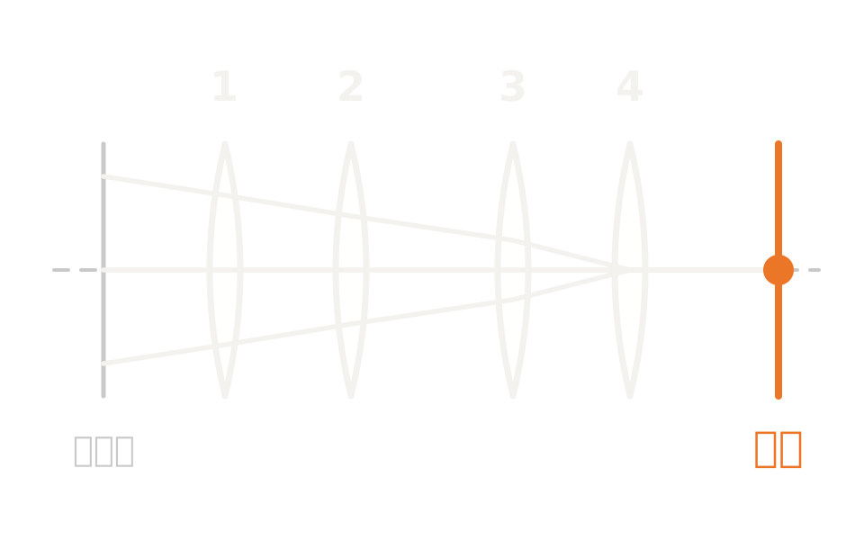
The surface-order assumptionRays travel from the object plane to the image plane, passing through each surface once in the defined order. They neither miss a surface nor strike the same surface twice.
A chain of local coordinatesThe position of each surface is given as the distance from the one before it, and the system is expressed as a chain of local coordinates.
Wavefront aberrationThe departure of the real wavefront at the exit pupil from the ideal reference sphere, defined as the optical path difference of real rays divided by the wavelength.
Decomposition of the aberrationsExpanding the wavefront aberration in field and pupil coordinates yields the classical aberration coefficients, and the residual is decomposed into Zernike polynomials and read term by term.

What the method is good at

Why this method is chosen

Computational cost is set by the number of surfaces

Because a single ray passes through each surface once, the number of intersection calculations is set by the number of surfaces. Large numbers of rays and large numbers of candidate designs can be evaluated in a short time.

Problems can be separated out as aberrations

By treating the optical path difference as a wavefront aberration and expanding it as a function of field and pupil, design problems can be separated out term by term — spherical aberration, coma, astigmatism and so on.

The model parameters are the design variables

Surface shapes, spacings and materials are quantities you can vary directly. They connect straight into an optimisation that drives the evaluated quantities towards their targets.

Where it fits

Where it fits, and where it does not

Where it fits

→ When the system is one in which light passes through surfaces in a fixed order — a photographic lens, a telephoto lens, a microscope, a telescope, a relay lens or a spectrometer

→ When evaluating the performance of an afocal system

→ When you want to set the quantities to be evaluated and optimise with the surface data as variables

→ When you want a first, approximate picture of ghost paths arising from double reflection

Where another method is the better fit

Systems whose surface order cannot be fixed: systems in which you cannot determine in advance which surface a ray strikes and in what order — prisms, corner cubes, light pipes, geometry imported from CAD — are handled by non-sequential ray tracing. The dividing line is not whether reflection is present, but whether the order can be fixed.

Exhaustive coverage of stray-light paths: a trace that assumes surface order can only give an approximation as far as double reflection. Evaluating paths exhaustively belongs to stray light analysis.

Coherent fields: where the amplitude and phase at intermediate surfaces are themselves required, physical optics propagation is the better fit.

The effect of manufacturing variation: to see the spread of performance against error rather than at nominal values, the work is set up as a tolerance analysis.

Applications

Typical applications

Camera and imaging optics

Designing the imaging performance of photographic and telephoto lenses.

Metrology optics

Refining the imaging performance of microscopes, telescopes, relay lenses and spectrometers.

AR/VR optics

Used for the design and aberration correction of eyepiece optics.

Evaluation coupled with structural and thermal analysis

Mapping deformation obtained from thermal or structural analysis onto the surfaces and evaluating the resulting change in performance.

Inputs and outputs

What you supply, and what you get back

INPUT

Surface data Radius of curvature, thickness, material, semi-diameter, conic constant
System conditions Aperture, field points, wavelengths
Variables Which surface data the optimisation is allowed to vary
Merit function The set of operands expressing the targets and constraints

OUTPUT

Geometric measures Spot diagrams, and tangential and sagittal ray aberration plots
Wavefront Wavefront aberration expressed as optical path difference
Measures that include diffraction MTF by the FFT and Huygens methods, and the diffraction point spread function
Image evaluation Geometric image simulation, and image simulation including diffraction

How it is done

How the work actually proceeds

01

Enter the surface sequence

Give each surface a radius of curvature, thickness, material and clear aperture, and set the aperture, field and wavelengths.

02

Choose the variables and the merit function

Mark the surface data to be varied as variables, and build a merit function expressing the targets and constraints.

03

Run the optimisation

Run a local optimisation that reduces the merit function, and inspect the converged solution.

04

Re-evaluate the result

Compare spot size, optical path difference and MTF before and after optimisation, and return to the merit function if needed.

How the merit function is built very largely determines the outcome of the optimisation. Step 02 is where most of the time should go.

Comparison with related methods

Choosing between related analysis methods

Method Relationship Main subject How they divide up
Sequential ray tracing (this method) This method Imaging systems whose surface order can be assumed Traces on the assumption that each surface is passed once and in order, running aberration evaluation and optimisation quickly.
Non-sequential ray tracing Alternative Systems whose paths are determined by geometry Intersections are determined solely by the position and properties of the objects and the direction of the ray. A ray may strike the same object any number of times.
Physical optics propagation (POP) Complementary Propagation of a coherent field Rays in a spot diagram do not interfere with one another. Where a field in which amplitude and phase interfere is required, this is the method to use.
Tolerance analysis Downstream The effect of manufacturing variation Takes the optimised nominal design directly as input and estimates the spread of performance against error, and the resulting yield.
Stray light analysis Downstream Exhaustive evaluation of unintended paths A trace that assumes surface order yields only an approximation as far as double reflection. The design is converted, and the work moves on to an evaluation that covers paths exhaustively.

View all analysis technologies →

Available in

The product that provides this method

Sequential ray tracing is provided as one of this product’s analysis modes. Editing surface data, optimising against a merit function and running a tolerance analysis are all handled in the same environment. See here for licensing, system requirements and adoption.

Ansys Zemax OpticStudio

View the product page →

FAQ

Frequently asked questions

Can afocal systems be handled?Yes. Afocal systems, like imaging systems, are handled in the same framework as systems whose surface order can be assumed.
How is the point spread function including diffraction obtained?The FFT point spread function assumes a large F-number, so that scalar diffraction theory holds, little distortion of the exit pupil, and a chief ray arriving very nearly normal to the image plane. Where the image plane is tilted, the exit pupil is distorted, or polarisation has to be taken into account, the Huygens point spread function is used instead.
Can imaging performance be judged from the spot diagram alone?No. A spot diagram is a collection of per-ray intersection points and does not include interference between rays. In a system whose aberrations are small enough, diffraction dominates, so the spot diagram is checked alongside the MTF and the point spread function including diffraction.
Can this be linked to tolerance analysis and to thermal or structural analysis?Yes. The optimised nominal design can be passed straight to a tolerance analysis. There is also a route for mapping loads or deformation obtained from thermal or structural analysis onto the optical surfaces and evaluating the resulting change in performance.

Reference information

Last updated

2026-08-18

Technical review

LightBridge Technical Support

Sources consulted

Ansys Zemax OpticStudio 2025 R1 User GuideExploring Sequential Mode in OpticStudio (Ansys Optics Knowledge Base)Exploring Non-Sequential Mode in OpticStudio (Ansys Optics Knowledge Base)What is a Point Spread Function? (Ansys Optics Knowledge Base)How to design a singlet lens, Part 3: Optimization (Ansys Optics Knowledge Base)

Talk to us about the design and analysis of imaging optics

Tell us what you are designing and the characteristics you want to evaluate, and we will suggest the appropriate method and approach.