Home/Analysis Technologies/Optical design/Tolerance Analysis

Analysis Technologies | Optical Design

Tolerance Analysis

A method that determines how far the errors specified as tolerances shift performance, from per-item sensitivity and from statistical samples generated according to a tolerance model.

Target

Manufacturing and assembly errors

Method

Sensitivity analysis and Monte Carlo analysis

Supporting products

Ansys Zemax OpticStudio

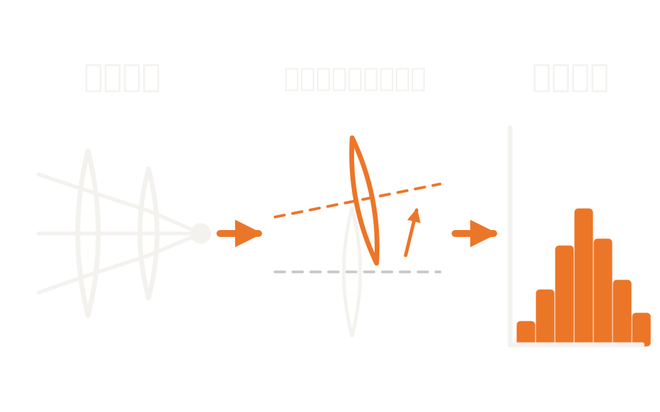
Schematic showing several samples of a nominal optical system with errors applied, and the resulting performance distribution

What the method is

Building the case for the tolerances on the drawing

Tighten the tolerances and performance is preserved, but machining and assembly cost more. Loosen them and cost falls, but more units miss the specification. Where to tighten and where you can afford to loosen cannot be decided without knowing the sensitivities.

Sensitivity analysis takes each toleranced item one at a time, moves it to its maximum and minimum, and extracts the change in a reference merit per item. Monte Carlo analysis samples every toleranced item per trial according to the tolerance model and its statistical distribution you have defined, giving the statistical distribution of performance and the yield.

Which element is moved at assembly to recover performance can also be included in the evaluation as a compensator. Where adjustment is assumed, looser tolerances can sometimes still meet the specification.

How it works

Per-item sensitivity, and simultaneous sampling from distributions

Sensitivity analysis applies the extreme values of each tolerance one item at a time and computes the change in the reference merit. What you get is the contribution per item, readable as a ranking of which errors matter. Because extremes are applied one at a time by construction, interaction between several errors occurring together is not included.

Monte Carlo analysis generates statistical samples according to the tolerance model you have defined. In one trial, every toleranced item is set at random from its allowed range and distribution. Repeating trials gives the statistical distribution of production performance and the fraction meeting the specification. The distribution can be normal, uniform or parabolic, the default being a normal distribution spanning four standard deviations between the maximum and minimum of the allowed range. Rather than a calculation that moves all items at once, it is an analysis whose result is decided by which distribution you assume.

One factor at a timeSensitivity analysis applies the extreme values of each tolerance one at a time and extracts the change in merit per item. Interaction between items is not included.
Sampling from the tolerance modelMonte Carlo analysis sets every toleranced item at random from its allowed range and distribution, once per trial, and evaluates performance in that state.
The assumed distributionBy default a normal distribution spanning four standard deviations between the maximum and minimum of the allowed range is used. Uniform and parabolic distributions can be chosen instead.
Solving it the other way roundYou can also set an upper bound on the merit first and find the loosest tolerance values that still meet it. That is the direction for reducing cost.

Strengths of this method

Why this method is chosen

Contributions can be separated

Moving one item at a time shows which errors matter, as a ranking. Which items to tighten and which to loosen can be separated with evidence behind it.

Production expressed in numbers

Sampling every toleranced item from its distribution and repeating trials gives the statistical distribution of performance and yield as the fraction meeting the specification.

Assembly adjustment can be built in

Elements that can be moved at assembly can be given as compensators, so performance can be evaluated realistically on the assumption of adjustment.

Where it fits

Where it fits, and where it does not

Where it is a good fit

→ when you want to estimate as-built performance before handing a nominal design to manufacturing

→ when you want to identify which error items should be tightened

→ when you want to know the fraction meeting specification, the yield, at the design stage

→ when the performance limit is fixed and you want the loosest tolerances that meet it

→ when you want the variation of a system evaluated on detector values, such as an illumination or stray light system

Where another method is the better fit

Building nominal performance: raising performance itself with no errors applied is handled by optimization against a merit function.

Deformation from heat or structure: deformation from physical loads rather than manufacturing variation has its own route, mapping thermal and structural results onto the optical surfaces. That is handled differently from statistical tolerances.

Evaluating unintended paths themselves: breaking down the contribution of scattering and ghosting path by path is the territory of stray light analysis.

Process variation in photonic circuits: process variation in photonic integrated circuits is the territory of a circuit-level analysis environment.

Applications

Typical applications

Cameras and imaging optics

Study tolerance allocation and yield for production lenses.

Spectrometers

Settle the tolerance allocation that guarantees measurement accuracy.

Systems with tilt and decenter

Apply element tilt and decenter as coordinate offsets and evaluate their effect.

Illumination and stray light evaluation

Use detector values as the merit function to see the variation of a system that assumes no path.

Inputs and outputs

What you provide, and what you get

INPUT

Nominal design The design data after optimization
Tolerance items Radius of curvature, thickness, surface decenter and tilt, element decenter, refractive index, Abbe number and more
Statistical conditions The allowed range and distribution per item, and the number of Monte Carlo trials
Merit and compensators The reference merit, and the elements available as compensators with their ranges

OUTPUT

Sensitivity The change in merit at the extreme values, per item
Allowed values The loosest tolerance value per item that still meets the limit you set
Statistical distribution The performance distribution and yield from Monte Carlo analysis
Perturbed models The design data generated for each trial. A poor unit can be opened and its cause traced

How it works

How it works in practice

01

List the tolerance items

Enumerate radius of curvature, thickness, decenter and tilt, refractive index and element tolerances, and tidy up items that duplicate one another mechanically.

02

Match tolerance values and distributions to reality

Give the allowed ranges from what your machining supplier and assembly process actually achieve. If the default distribution does not match the reality of the process, change it.

03

Define the compensators

Specify the elements that can be moved at assembly and their adjustment ranges, and confirm they are working as intended.

04

Run sensitivity and Monte Carlo analysis

Identify the dominant items, then repeat trials according to the tolerance model to obtain the statistical distribution of performance and the yield.

If the compensators are set up unrealistically, the yield comes out higher than it really is. Step 03 is where most of your time should go.

Comparison with related methods

Choosing between related analysis methods

Method Relationship Main targets When to use which
Tolerance analysis (this method) This method Manufacturing and assembly variation Quantifies the effect of errors through per-item sensitivity and a statistical distribution following the tolerance model, and estimates yield.
Sequential Ray Tracing Upstream Imaging performance at nominal values Optimizes the nominal design that is the input to tolerance analysis. Settle nominal performance first, then apply errors.
Non-Sequential Ray Tracing Upstream Systems evaluated on detector values Provides the model for a system that assumes no path. The reference is a user-defined merit function rather than a built-in metric.
Stray Light Analysis Complementary The contribution of unintended paths Tolerance analysis handles the variation of intended performance; stray light analysis handles the contribution of unintended paths. They address different things.
Lumerical INTERCONNECT Alternative Process variation in photonic circuits Variation in photonic integrated circuits is handled at circuit level. That is a different subject from lens system tolerancing.

View all analysis technologies →

Supporting products

Products that provide this method

Tolerance analysis is an analysis capability built into this product. It applies both to systems assuming surface order and to systems assuming no path, and the merit function used for optimization can be used directly as the reference. See here for licensing, system requirements and deployment.

Ansys Zemax OpticStudio

View the product page →

FAQ

Frequently asked questions

Which comes first, sensitivity or Monte Carlo analysis?Normally sensitivity analysis. Identify the dominant items, adjust the tolerance values, then look at the production distribution and yield with Monte Carlo analysis. There is also a setting to skip sensitivity analysis and go straight to Monte Carlo.
What distribution is assumed?By default a normal distribution spanning four standard deviations between the maximum and minimum of the allowed range. That is an assumption, not a measurement of your process. If your actual process differs, change it to a uniform or parabolic distribution.
What is compensation?The operation of moving a particular element at assembly to recover performance. In the analysis you specify a range as a compensator and evaluate performance after that adjustment. The adjustment method can be running an optimization, moving only the back focus, or applying no compensation at all.
Can tolerance analysis be run on a system that assumes no path?Yes. Tolerance items are provided for object position and tilt, object parameters and materials. The reference is a user-defined merit function, though, and compensator limits are ignored, so ranges are given as constraints within the merit function instead.

References

Last updated

2026-08-18

Technical review

LightBridge Technical Support

Sources consulted

Ansys Zemax OpticStudio 2025 R1 User Guide (Tolerancing)How to perform a sequential tolerance analysis (Ansys Optics knowledge base)How to perform a Non-Sequential tolerance analysis (Ansys Optics knowledge base)How to design a singlet lens, Part 3: Optimization (Ansys Optics knowledge base)

We can advise on how to allocate tolerances

Tell us the design data and the specification you need to hold, and we will propose how to run the tolerance analysis.