A practical workflow for designing and analysing centimetre-scale metalenses across Lumerical and Zemax OpticStudio: building a meta-atom database with RCWA, exchanging data through HDF5, ray tracing, and exporting GDS.
Published
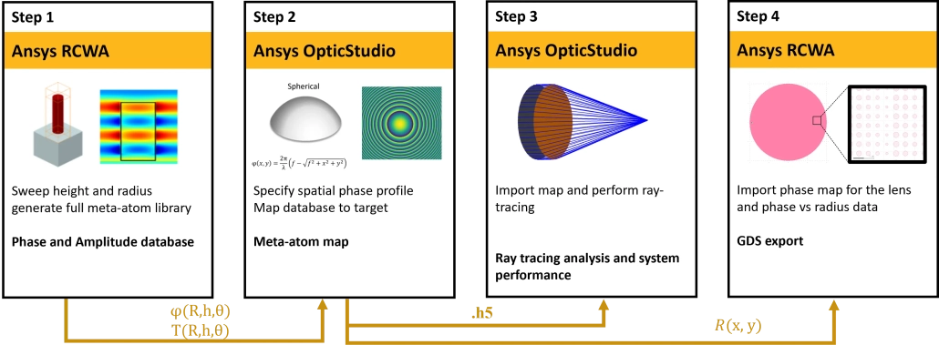
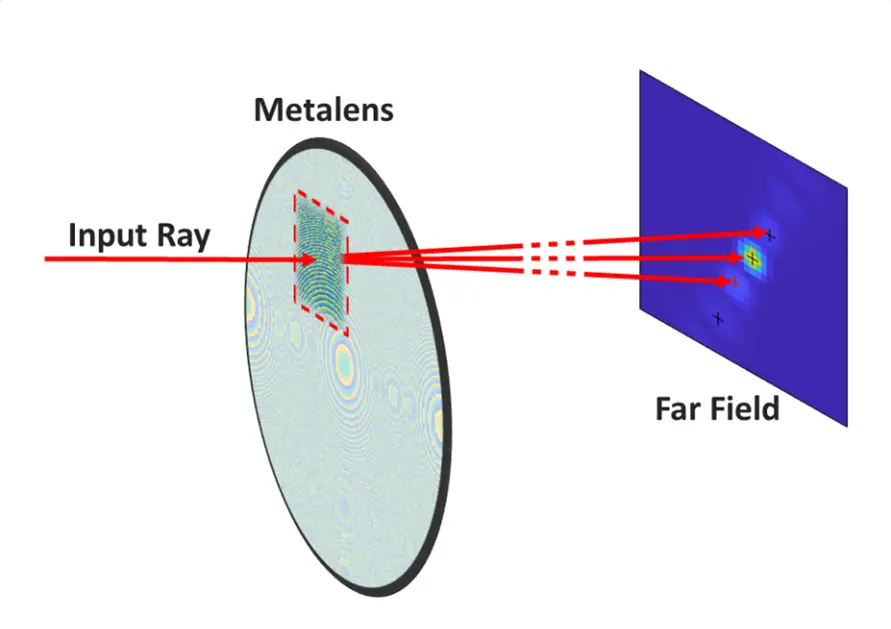
This article presents a simulation workflow for designing a centimetre-scale metalens. The nano-elements are modelled in Lumerical, and the RCWA method is used to build a database of the phase and amplitude induced by a single cell as a function of radius. That data is exported to OpticStudio and integrated into a ray-tracing system in which a collimated beam is focused by the metalens.
Note: this feature is available only in Ansys Zemax OpticStudio Premium and Enterprise. Generating the .h5 file requires Ansys Lumerical version 2023 R2 or later. Multi-wavelength simulation is supported only by plugin version 2025 R1 or later.
Overview
A metalens is an advanced optical structure built from nano-elements. Tuning individual cells locally makes complex optical functions possible. Simulating this kind of device at scale, however, is a considerable challenge: a metalens is not a periodic structure, and it is made up of a very large number of nano-elements. A metalens is also fundamentally a wave-optics device, yet it has to be integrated into a ray-tracing system.
How the metalens is created and how the RCWA calculation is validated are covered in the article “Metalens Design Across Lumerical and Zemax: Design Flow and Validation Guide“. That workflow deals with a relatively small metalens and suits simulating beam propagation through the optical system with the Physical Optics Propagation (POP) tool in OpticStudio. That method limits the lens size that can be simulated, mainly because of the memory the calculation requires. This article presents a different workflow for designing a large metalens 10 mm in diameter. It shows how a metalens can be designed at the nano-element level and then assembled to a centimetre scale, after which the metalens is integrated into the ray-tracing system in OpticStudio. The same workflow lets users design larger metalenses according to their own requirements and compute resources. As an exercise after completing this workflow, we therefore recommend that users attempt a 20 mm diameter lens design, which will build familiarity with the workflow and an understanding of the key parameters in the simulation files. The process of extracting the metalens information as a GDS file for fabrication is also described.
Step 1: unit cell simulation, sweeping height and radius
In Lumerical, sweep the unit cell parameters (the nanorod radius, for example) to build a parametric database of the nano-element response. For more detail, see step 2 of the article “Metalens Design Across Lumerical and Zemax: Design Flow and Validation Guide”. This example builds a database of phase (phi) and transmittance (T) against nanorod radius R, height h and angle of incidence theta.
Step 2: defining the target phase and generating the nano-element map
Define the target phase profile of the metalens. At scales beyond a few hundred micrometres, the memory needed to generate, store and use a complete phase map becomes very large for a typical CPU. This workflow therefore uses target phase profiles that can be defined analytically, such as spherical or cylindrical surfaces. Ansys OpticStudio can also be used to optimise the desired wavefront at the metalens surface within the complete optical system, which lets the target phase be defined as a function with a discrete number of coefficients (a polynomial, for example). For examples of more advanced optimisation workflows, see “Eye tracking optical system with a metalens” or “Fiber Endoscope Design Using Metalens for Illumination and Collection“. This example creates a .h5 file that matches the target phase using data collected from the database. The nanorod radii R and their positions (x,y) are also saved as a .h5 file, which is used later in step 4 to create the GDS export file.
Step 3: integration into OpticStudio
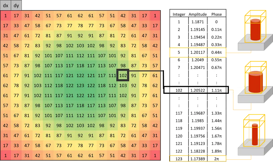
Define the large metalens from the target phase profile and the database defined in the previous steps. The database is written out as a file containing an index map, in which each cell references a list of discrete phase and amplitude values the index can take. That file is then used with the Zemax plugin included in the download package to integrate the large metalens into the ray-tracing system.
Step 4: GDS generation
GDS export is supported at this scale as well. For details, see the article “Metalens Design Across Lumerical and Zemax: Design Flow and Validation Guide”.
Running the workflow, and results
Step 1: unit cell simulation, sweeping height and radius
1. Run the script generate_meta-atom_database.lsf.
This step sweeps the cell parameters (the nanorod radius, for example) to determine the relationship between the local properties of the cell element and its output phase and amplitude. The procedure is unaffected by the final scale of the metalens. For more detail, see step 2 of the article “Metalens Design Across Lumerical and Zemax: Design Flow and Validation Guide”. The output file of this sweep contains the phase and amplitude database information and is named phase_amp_vs_radius_wave_theta_phi.h5.
Note that because the sweep runs over a discrete number of phases, the nanorod radii are also limited to a discrete set of values. That discretisation is reflected in the resulting phase, and it mirrors the natural manufacturing constraint on nano-elements: in practice only a fixed, discrete number of different meta-atoms can be fabricated.
RCWA solver parameters must also be set. The sweep runs over a particular spectral range and angular range. We recommend making the angular range cover the maximum expected angle of incidence, and making the spectral range include the design wavelength at which the target phase is defined.
Step 2: defining the target phase and generating the nano-element map
In a real design, Ansys Zemax OpticStudio can be used to derive the desired phase function through an optimisation process. For details of that process, see the appendix below and “Eye tracking optical system with a metalens” or “Fiber Endoscope Design Using Metalens for Illumination and Collection“. Because this example uses a simple phase function that can be defined analytically, a simple function defined directly in a Lumerical script is sufficient.
Generating a 20 mm diameter metalens can take some time. We therefore recommend trying the workflow once with a smaller lens first, for example 10 mm in diameter with a 25 mm focal length.
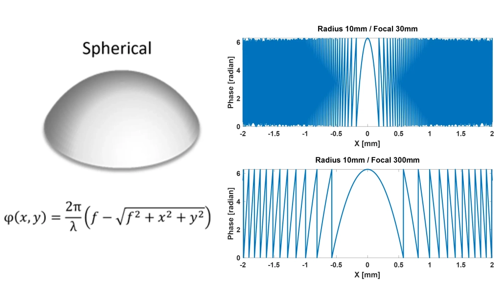
2. Open the script generate_metalens_data.lsf, set the lens type to "spherical", specify the focal length and lens radius, then run Part 1 and check the one-dimensional profile.
When working with a lens several millimetres in diameter at a nanoscale resolution set by the size of the nano-elements, generating a file containing the complete map of the target phase may require a great deal of memory. Instead, this workflow restricts itself to phase maps that can be described by an analytic function. This article targets a spherical lens of 5 mm radius and 25 mm focal length.
Note that it is important to keep the numerical aperture (NA) at a sensible value. If the metalens is designed to a very fast lens profile, the phase variation at the edge of the lens may exceed what the resolution of the nano-elements can achieve. To secure a 2*pi phase range between unit cells, the numerical aperture must satisfy the Nyquist sampling criterion [1] shown below.
Here p is the unit cell size, lambda is the design wavelength and NA = radius / focal length. Beyond this fundamental limit the gradient of the wrapped phase becomes too steep, producing abrupt jumps when the local phase gradient method is used, so the metalens model is expected to be limited. For details, see the discussion in the appendix.
Generating the phase map in Lumerical
3. Run Part 2 of the script generate_metalens_data.lsf.
4. Copy the .h5 file generated by the script into the Zemax > DLL > Surfaces folder.
The centimetre-scale lens is defined from the target phase profile and the phase library defined in the previous steps. The .h5 file contains an index map structured so that each cell references a list of discrete phase and amplitude values. Each index points to an entry in the list of possible phase and amplitude values, and each entry corresponds to a nanopillar characterised by its radius.
Note also that the phase and amplitude database is calculated for each angle of incidence defined in the RCWA object. Checking the parameters on the “Excitation” tab of the RCWA solver shows that this example runs the RCWA calculation over an incidence angle range of 0 to 40 degrees. The phi range matters too: phi must be set either over the range -180 to 180 degrees, or as the single value phi=0.
The database of amplitude and phase values does not itself depend on the scale of the lens, but the index map grows as the lens gets larger. File size grows in proportion to the number of nano-elements in the design, so we recommend a provisional test with a smaller diameter lens first. For oblique incidence the database covers a wider range of values still, since different angles of incidence must be accounted for. For details see the related article. A single averaged unit cell value is sufficient to represent the phase and amplitude response. This downsampling is described in step 2 of the article “Metalens Design Across Lumerical and Zemax: Design Flow and Validation Guide“.
Step 3: integration into OpticStudio
5. Open the file metalens_10mm.zprj.
6. Check the system parameters.
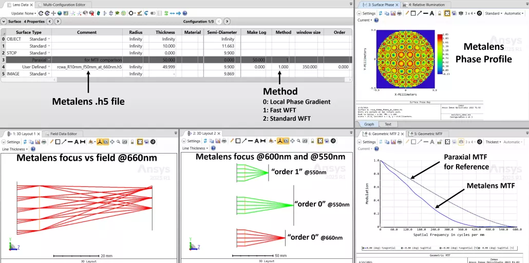
    1. The .h5 file is set in the Comment column of the metalens surface.
    2. The Method selected on the metalens surface is set to 1. This is the recommended method; see the appendix for details.
    3. Two different wavelengths are considered in the Multi-Configuration Editor. For 550 nm, two different diffraction orders are selected.
The metalens is set up in OpticStudio as a User Defined Surface using the DLL lumerical-metalens-XXXX.dll, where “XXXX” is the version and timestamp. The data is then loaded by entering the name of the generated .h5 file, including its extension, in the Comment column. For a 20 mm diameter metalens, loading the data can take some time.
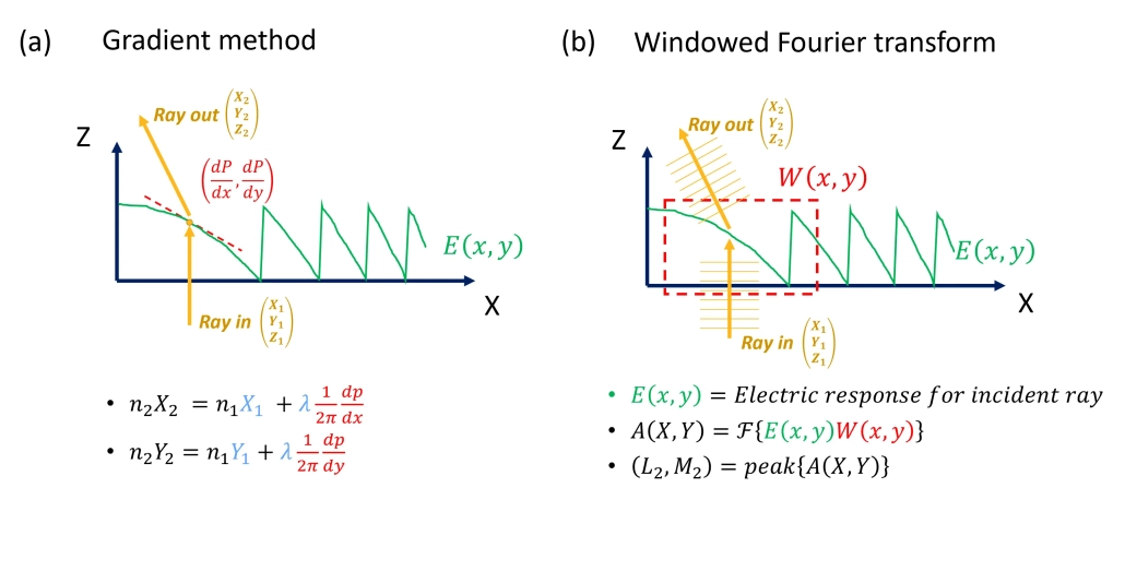
Two different methods are available for calculating the outgoing direction of a ray after it interacts with the metalens element. The choice is made with the “Method” parameter: a value of 0 selects the local phase gradient method, and 1 or 2 select the Windowed Fourier Transform (WFT) method at different accuracy levels. The difference between the two methods is explained in the appendix.
The WFT method is used by default, because it is more accurate and can also analyse several diffraction orders.
Compared with the local phase gradient method, the WFT method lets you choose which diffraction order to use. Note that “order” in this context may not correspond exactly to the standard definition of diffraction order. The peaks detected in angular space are ordered by decreasing intensity, so “Order 0” corresponds to the order with the most energy. If the order parameter is larger than the number of peaks detected, the last order (the weakest peak) is used.
Step 4: GDS generation
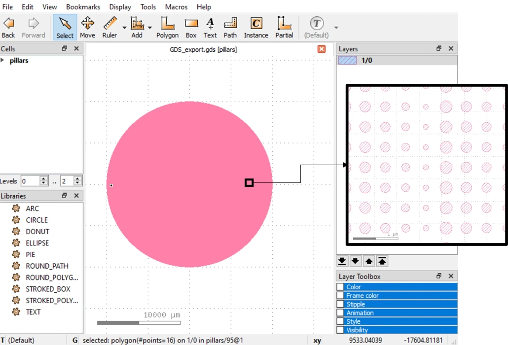
7. Open the script gds_export.lsf. Set the focal length to 25 mm and the lens radius to 5 mm, then run the script.
Export to GDS format is the important final step for fabrication. This feature is supported at this large scale as well. For details, see the article “Metalens Design Across Lumerical and Zemax: Design Flow and Validation Guide“.
Important model settings
A description of the important objects and settings used in this model
Even with this latest workflow, the maximum size that can be simulated is limited by the RAM of the computer. With 64 GB of RAM, the largest metalens that can be generated is one of a little over 10 mm radius.
At present only polarisation-independent meta-atoms are supported in ray tracing.
A metalens is built from unit cells of finite size, and the phase library is generated with discrete phase values. The f-number of the lens must therefore be set so that the variation of the phase profile does not exceed what the resolution of the unit cell can achieve.
The two methods for determining the outgoing ray direction are also calculated from the local profile around the position where the ray strikes the metalens, so accuracy may fall at the edge of the lens where part of the surrounding region lies outside the metalens. Rays striking the edge of the lens may therefore not be refracted as expected. We recommend setting the aperture size slightly smaller than the actual size of the metalens. In this example the metalens is 20 mm in diameter while the system aperture diameter is set to 19.8 mm. Using “Entrance Pupil Diameter” as the aperture type is also recommended to secure the correct metalens size.
In the RCWA sweep that generates the meta-atom database, the phi angular range must also be set either to 0 alone or to cover the range -pi to pi.
Updating the model to your own parameters
How to update the model for your device parameters
The focal length, lens size and phase function defined in step 1 can be customised to generate metalenses with different functions.
When optimising a metalens in Zemax OpticStudio, the target metalens phase profile is normally defined using a Binary 2 surface (see How to model diffractive optics using the Binary 2 surface for details). In that case, set the lens type to “Binary2” in step 2. Then copy the normalised radius and Binary 2 coefficients optimised in Zemax and paste them into ‘norm_radius' and ‘zemax_coeffs' in the script.
This example uses the nanorod radius as the primary parameter for generating the desired phase. You can also define a different custom unit cell and include parameters such as height or duty ratio in the sweep, generating a database library as shown in step 2.
When running the RCWA sweep, the database can be generated quickly with few sample points over the meta-atom parameters (radius at 10 nm intervals, for example). Where the phase can be assumed to vary relatively smoothly with the meta-atom parameters, spline interpolation is then used to interpolate the database more finely (sampling radius at 1 nm intervals, for example). If the variation is not smooth, it may be better to run the sweep directly with more sample points and change the interpolation from spline to linear, or to use no interpolation at all. This matters particularly when the meta-atom size approaches a resonance, where the amplitude profile can develop a deep dip.
Taking the model further
Information and tips for users who want to customise the model further
The .h5 file contains only the wrapped phase information. That corresponds to the physical structure of the metalens, which normally covers a 0 to 2*pi phase range within the range of the meta-atom parameters alone. Wrapped phase is sufficient for the ray refraction calculation, because the first method uses only the phase gradient, and phase wrapping does not affect the WFT calculation either. For further analysis such as OPD (optical path difference), however, there is an advantage in unwrapping the phase. Phase unwrapping is not straightforward, so this model provides an option to set a reference phase profile, which lets Zemax unwrap the metalens phase profile correctly. This option is available only when the local phase gradient method is selected, that is when Method = 0. The reference phase map is defined by the expression below.
where
For a simple spherical profile such as the one in this example, the expression becomes:
Enabling this option makes it possible to visualise the unwrapped phase using the “Surface Phase” analysis tool.
Further material
Related papers
Mu Ku Chen, Yongfeng Wu, Lei Feng, Qingbin Fan, Minghui Lu, Ting Xu, and Din Ping Tsai “Principles, Functions, and Applications of Optical Meta-Lens”, Advanced Optical Materials, Volume 9, Issue 4 (January 2021); https://doi.org/10.1002/adom.202001414
T. Leportier, D. Bacon-Brown, D. McGuire, S. Gangadhara, B. Williams, M. George, A. Reid, “Novel workflow for metalens optical system design, simulation, and manufacture,” Proc. SPIE 13373, Photonic Instrumentation Engineering XII, 133730R (19 March 2025); https://doi.org/10.1117/12.3040737
Han-Hsiang (Michael) Cheng, Thibault Leportier, Dan-Nha Huynh, Jens Niegemann, Adam Reid, Wei-Hsin Chen, “Ray-tracing compatible methods for large-scale metalenses in multiwavelength imaging system,” Proc. SPIE 13378, High Contrast Metastructures XIV, 1337809 (19 March 2025); https://doi.org/10.1117/12.3040478
Appendix
Supplementary information and theory
Two different propagation methods are available for calculating the direction of the outgoing ray after it interacts with the metalens.
Local phase gradient method
The local phase gradient method applies when the “Method” parameter is set to 0. This method interpolates the phase values around the position where the ray strikes the metalens to obtain the local phase gradient at that position, and from that gradient the outgoing direction of the m-th order diffracted ray is calculated by the expression below.
where (Xi, Yi, Zi) are the unit vectors of the incoming and outgoing rays, n1 and n2 are the refractive indices of the incident and exit media, lambda is the wavelength, m is the diffraction order and P(x,y) is the local phase in radians. The z direction is assumed to be the surface normal.
Two interpolation methods are available for calculating the ray bending from the phase gradient, selectable in the OpticStudio surface parameter. A value of 1 is bilinear interpolation and 3 is bicubic interpolation. Bicubic interpolation is slightly more accurate, while bilinear interpolation is expected to be more stable against phase jumps.
Windowed Fourier Transform (WFT)
The WFT method applies when the “Method” parameter is set to 1 or 2, corresponding to the “fast” and “standard” settings respectively. Method = 1 is normally recommended, on grounds of both speed and accuracy. The basic principle of the WFT method is to treat the ray striking the metalens as a local plane wave. A window function is applied to the metalens profile (phase and amplitude) and an FFT is then performed to obtain information in angular space. Each diffraction order produced by the metalens appears as a peak in angular space. Detecting the positions of these peaks in angular space gives the outgoing direction of the ray after interacting with the metalens.
One of the important factors in this method is the window size. Accuracy in angular space is inversely proportional to the window size, so the window must be set large enough. An FFT calculation is performed for every ray, however, so too large a window slows the calculation. When Method 1 or 2 is selected, a parameter is available for setting the window size in units of lambda. The default is 100 lambda, but as a rule of thumb we recommend setting it to about .
Method 1 is a fast WFT implementation with advanced parameters for window selection. It is expected to be fast enough and accurate enough to give MTF results that match experimental measurement. Method 2 is a more standard WFT implementation. It is considerably slower and becomes unwieldy for window sizes above 150 lambda, but it is provided for the special cases where other implementations behave unexpectedly.
Notes on comparing the methods
The local phase gradient method is relatively simple to compute and therefore fast, which suits the initial design stage or a quick evaluation at a single wavelength. At wavelengths other than the design wavelength, however, this method may not give accurate results. One reason is that at a different wavelength the phase jumps produced by the metalens structure no longer coincide with 0 to 2*pi phase jumps, so the periodicity of the phase jumps no longer matches the underlying phase profile. The WFT method, by contrast, gives more accurate results at wavelengths other than the design wavelength. It can also handle several diffraction orders, which allows more detailed analysis of the system. The accuracy of the results (MTF in particular) can depend on the window size chosen.
We may request cookies to be set on your device. We use cookies to let us know when you visit our websites, how you interact with us, to enrich your user experience, and to customize your relationship with our website.
Click on the different category headings to find out more. You can also change some of your preferences. Note that blocking some types of cookies may impact your experience on our websites and the services we are able to offer.
Essential Website Cookies
These cookies are strictly necessary to provide you with services available through our website and to use some of its features.
Because these cookies are strictly necessary to deliver the website, refusing them will have impact how our site functions. You always can block or delete cookies by changing your browser settings and force blocking all cookies on this website. But this will always prompt you to accept/refuse cookies when revisiting our site.
We fully respect if you want to refuse cookies but to avoid asking you again and again kindly allow us to store a cookie for that. You are free to opt out any time or opt in for other cookies to get a better experience. If you refuse cookies we will remove all set cookies in our domain.
We provide you with a list of stored cookies on your computer in our domain so you can check what we stored. Due to security reasons we are not able to show or modify cookies from other domains. You can check these in your browser security settings.
Google Analytics Cookies
These cookies collect information that is used either in aggregate form to help us understand how our website is being used or how effective our marketing campaigns are, or to help us customize our website and application for you in order to enhance your experience.
If you do not want that we track your visit to our site you can disable tracking in your browser here:
Other external services
We also use different external services like Google Webfonts, Google Maps, and external Video providers. Since these providers may collect personal data like your IP address we allow you to block them here. Please be aware that this might heavily reduce the functionality and appearance of our site. Changes will take effect once you reload the page.
Google Webfont Settings:
Google Map Settings:
Google reCaptcha Settings:
Vimeo and Youtube video embeds:
Other cookies
The following cookies are also needed - You can choose if you want to allow them:
Privacy Policy
You can read about our cookies and privacy settings in detail on our Privacy Policy Page.