Home/Analysis Technologies/Electromagnetic analysis/RCWA

Analysis Technologies | Electromagnetic Analysis

RCWA (Rigorous Coupled-Wave Analysis)

A semi-analytic method for layered structures with in-plane periodicity. The fields are expanded in the Fourier domain and solved analytically layer by layer, and those solutions are then connected to give the response per diffraction order.

Formulation

Semi-analytic expansion in the Fourier domain

Problem solved

Layer-by-layer solutions connected by scattering matrices

Supporting products

Lumerical FDTD

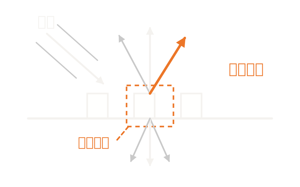
$Diagram showing a plane wave incident on a periodic unit cell, with the solutions obtained layer by layer emerging as diffraction orders$

What the method is

Assume periodicity, obtain the response per order

RCWA obtains the optical response of a plane wave incident on a multilayer structure by solving Maxwell’s equations semi-analytically. It applies to structures whose layer geometry varies periodically in-plane, such as photonic crystals and diffraction gratings.

The calculation has three stages. First the structure is divided into a series of layers uniform along the propagation direction. Then Maxwell’s equations are solved analytically in the Fourier domain within each layer; the wave vectors of the Fourier modes are called k-space vectors. Finally the layer solutions are propagated in both directions and connected to give the scattering matrix of the whole structure.

Two quantities decide the accuracy: the number of layers the cross-section is divided into, and the number of k-space vectors retained. Increasing either raises accuracy and increases run time.

How it works

Solved analytically layer by layer, connected by scattering matrices

The premise of the method is that the same geometry repeats in-plane. The in-plane width of the analysis region defines the unit cell boundary, and outside it the same geometry is taken to continue periodically. Because there is a period, the in-plane fields can be written as a Fourier series. Truncating what is really an infinite expansion at a finite number of terms is what makes it a numerical problem of manageable size.

The truncation is specified by selecting k-space vectors in order of proximity to the origin. The shape of the selection region can be circular or rectangular. For two-dimensional calculations there is also a setting for how the series is handled at surfaces where permittivity changes discontinuously. Because neither a spatial grid nor a time step is used, there is no grid-induced numerical dispersion and no staircased geometry.

Unit cellThe in-plane width of the analysis region defines the unit cell boundary. Outside it the same geometry is taken to continue periodically.

Division into layersThe structure is divided into a series of layers uniform along the propagation direction. The more layers, the finer the representation of slanted sidewalls and curved surfaces.

Fourier expansionMaxwell’s equations are solved analytically in the Fourier domain within each layer. The number of k-space vectors retained sets the degree of truncation.

ConnectionThe layer solutions are propagated in both directions and connected to build the scattering matrix of the whole structure.

Strengths of this method

Why this method is chosen

What being semi-analytic gives you

RCWA and the analytic multilayer solution usually finish faster than solving the same problem in the time domain. A time-domain solver is fully numerical, whereas RCWA is semi-analytic, so for the same structure the time-domain result is generally the less accurate of the two.

Fewer quantities to tune

Only two quantities are varied for convergence: the number of layers and the number of k-space vectors retained. The setup itself is far simpler than a time-domain analysis.

Complex quantities per order

As well as the fraction of power in each diffraction order, you can extract complex scattering parameters resolved by polarization, and the complex amplitudes at the interfaces outside the layer stack.

Where it fits

Where it fits, and where it does not

Where it is a good fit

→ when you need diffraction efficiency per order for a layered, in-plane periodic structure

→ when you want to sweep angle of incidence and wavelength widely to study the dependence of the response

→ when you want to sweep unit cell dimensions and build a table mapping phase to transmittance

→ when you are handling geometry that can be represented as layers, such as a grating with slanted sidewalls

→ when you want to handle a thick periodic structure defined as repeated layers

Where another method is the better fit

Structures where periodicity cannot be assumed: the method assumes the same geometry continues outside the analysis region. If you need the effect of finite size itself, or arbitrary geometry with no period, you need a time-domain method that discretizes the volume.

Multilayer stacks with no in-plane pattern: if the layers are flat and laterally uniform, the analytic solution that multiplies matrices together is simpler and needs no convergence check.

Structures that emit light: the RCWA solver has no dipole source option and currently cannot be used for emitting structures.

Loss in the incident or exit layer: loss in the first and last layers is not currently supported. Where that applies, choose another method.

Applications

Typical applications

Meta-atom library generation

Sweep the unit cell dimensions and build a table mapping phase to transmittance. The procedure rests on the approximation of treating each cell as periodic.

Surface relief gratings

For gratings used in a waveguide, obtain the efficiency per order as a function of angle of incidence and wavelength.

Photonic crystal slabs

Obtain reflection and transmission spectra of a periodic slab as a function of frequency, angle and polarization.

Volume holographic gratings

Define a thick periodic structure as repeated layers and handle it at a realistic computational cost.

Inputs and outputs

What you provide, and what you get

INPUT

Unit cell	The geometry and materials of the unit cell, defined by the in-plane width of the analysis region
Layer definition	The boundary positions of the layers along the propagation direction. For thick periodic structures, layer repetition can also be specified
Solver settings	The shape of the region from which k-space vectors are selected (circular or rectangular), and the maximum number retained
Excitation conditions	How frequencies are laid out, angle of incidence and azimuth, s- and p-polarization, forward or backward
Lattice vectors	The angle of the lattice vectors when a non-orthogonal unit cell is used

OUTPUT

Total energy	The fraction of power going to reflection and transmission, per polarization
Diffraction orders	The fraction of power per order. Alternative normalizations are also available
Characterization per order	Complex scattering parameters per order, separated into s- and p-polarization
Amplitudes	The complex field amplitude per order at the interfaces outside the layer stack, and the forward and backward mode amplitudes in the upper and lower layers
Field distribution	Frequency-domain electric and magnetic fields on the grid, returned by a dedicated monitor

How it works

How it works in practice

Define the unit cell and the layers

Set the unit cell by the in-plane width and define the layer boundaries along the propagation direction. For thick periodic structures, use layer repetition.

Decide the k-space vectors to retain

Set the shape of the selection region and the maximum number. This is the setting that directly decides cost and accuracy.

Set the incidence conditions and outputs

Set how frequencies are laid out, the angle of incidence and azimuth, and the polarization, then choose the outputs you need. If internal fields are required, place a dedicated monitor.

Confirm convergence, then sweep

Increase the number of vectors and the number of layers and confirm the point at which the result stops moving, then move on to sweeping dimensions or angles.

Layer repetition and fully anisotropic materials each have feature combinations that cannot be used together. When using either, check first whether the combination is allowed. The RCWA solver is a feature of release 2023 R1 and later.

Comparison with related methods

Choosing between related analysis methods

Method	Relationship	Main targets	When to use which
RCWA (this method)	This method	Layered structures with in-plane periodicity	Solves each layer analytically in the Fourier domain and connects them to give the response per order. It rests on being able to assume periodicity.
STACK	Alternative	Multilayer stacks with no in-plane pattern	An analytic solution that multiplies layer matrices together. With no in-plane expansion it is simpler, and it needs no convergence check.
FDTD	Alternative	Structures where periodicity cannot be assumed	Discretizes the analysis region as a volume. Everything RCWA can solve can also be solved in the time domain, but RCWA usually finishes faster.
Non-Sequential Ray Tracing	Downstream	Carrying it into the whole system	Carry the grating response you obtained into a whole-system evaluation by ray tracing. Lumerical handles the fine structure and OpticStudio the whole system.

View all analysis technologies →

Supporting products

Products that provide this method

A commercial software environment for optical analysis of periodic and fine structures. Alongside a three-dimensional time-domain solver, rigorous coupled-wave analysis and the analytic multilayer solution sit in the same environment, so the same structure can be checked by a different method. See here for licensing, system requirements and deployment.

Lumerical FDTD

View the product page →

FAQ

Frequently asked questions

What exactly is rigorous about it?It means solving Maxwell’s equations without introducing an approximate physical model. Numerically there are two truncations: cutting the in-plane Fourier expansion at a finite number of terms, and dividing the structure into a finite number of layers. Those two decide the accuracy.

How many k-space vectors do I need?It depends on the structure; there is no generally applicable number. Increase the number selected in order of proximity to the origin and confirm the point at which the result stops moving. The same check is needed for the number of layers.

Can it be used for non-periodic elements?Not as it stands. For non-periodic elements such as a metalens, one approach is to treat each unit cell as periodic and obtain its response in advance. That approximation does not correctly capture coupling between neighboring cells, and it breaks down the more neighboring cells differ. Interaction across the whole element is handled by a time-domain calculation.

Can it handle emitting structures?No. The RCWA solver has no dipole source option and currently cannot be used for emitting structures. To handle emission within a layer, switch to the analytic multilayer solution for a flat stack, or to a time-domain method if there is an in-plane pattern.

Related technical information

The RCWA capability in Lumerical FDTD →

Optical sensor solutions →

Ray propagation in large-scale metalenses →

Guide to linking Lumerical and OpticStudio →

References

Last updated

2026-08-19

Technical review

LightBridge Technical Support

Sources consulted

Ansys Optics: RCWA Solver IntroductionAnsys Optics: RCWA Solver – Simulation ObjectAnsys Optics: RCWA Product Reference ManualAnsys Optics: RCWA Field Monitor – Simulation ObjectAnsys Optics: Photonic Crystal Slab (RCWA)Ansys Optics: Surface Relief Grating for Augmented Reality SystemAnsys Optics: Introduction to metalens workflowsAnsys Optics: Layer Repetitions in RCWA

We can advise on diffraction analysis of periodic structures

Tell us the make-up of the unit cell and the quantity you want to evaluate, and we will propose the method and product that suit.

Request a technical consultation