
Home/Analysis Technologies/Performance evaluation/MTF

Analysis Technologies | Performance Evaluation

MTF (Modulation Transfer Function)

A metric expressing how much of the contrast of a subject survives into the image, at each spatial frequency. It is the modulus of the optical transfer function, obtained from the Fourier transform of the point spread function, that is, the autocorrelation of the pupil function.

Definition

The modulus of the optical transfer function

Calculation methods

Three: FFT, Huygens and geometric

Supporting products

Ansys Zemax OpticStudio
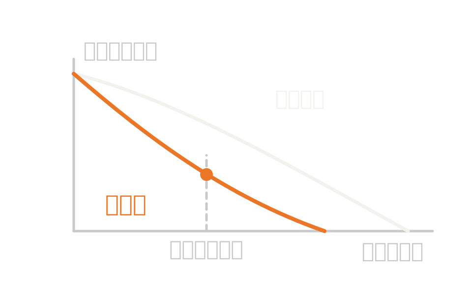
Diagram showing image contrast falling as spatial frequency rises, with the design curve below the diffraction limit curve

What the method is

The contrast that survives, frequency by frequency

When a subject with a sinusoidal light and dark pattern is imaged, the contrast of the image is lower than that of the subject. That ratio, as a function of spatial frequency, is the modulation transfer function. It is the modulus of the optical transfer function, defined as the normalized Fourier transform of the point spread function or the normalized autocorrelation of the complex pupil function. That definition is a standard result of Fourier optics.

OpticStudio uses that relationship directly as the route to the calculation. The point spread function follows from the wavefront data, and MTF is derived from the autocorrelation of the pupil function. The FFT calculation is based on an FFT of the pupil data, and the geometric calculation is performed as the Fourier transform of geometric spot data.

The horizontal axis is in cycles per millimeter in image space for a focal system, and cycles per milliradian in object space for an afocal system. Results are shown separately for the tangential and sagittal directions.

How it works

Obtained from the pupil data by three methods

The FFT method is fast but carries several premises: an f-number large enough for scalar diffraction theory to apply, the region where the point spread function has significant energy being small compared with the distance from exit pupil to image plane, the exit pupil not being greatly distorted relative to the entrance pupil, and sampling fine enough to represent the point spread function. For systems where the exit pupil is greatly stretched, switch to the Huygens method.

The Huygens method is not based on an FFT. The only premises it needs are an f-number large enough for scalar diffraction theory and sufficiently fine sampling. Use it for tilted image planes, greatly distorted exit pupils, arrangements where the chief ray cannot be traced, and summing across several configurations. The geometric method is an approximation to diffraction MTF and works where aberrations are large. Once the wavefront error exceeds about 10 waves, switch to the geometric method. It is also the only method that can include the loss of contrast from surface scattering.

FFT calculationObtained by FFT of the pupil data. Fast, but premised on being in the far field, the exit pupil not being greatly distorted, and the ray distribution in cosine space being nearly uniform.
Huygens calculationObtained from a point spread computed by direct integration of the Huygens wavefront. Because it does not depend on ray positions in the paraxial pupil, it carries fewer premises.
Geometric calculationObtained as the Fourier transform of geometric spot data. An approximation to diffraction MTF, and very fast for systems with large aberrations. There is also a setting to multiply by the diffraction limit curve to bring it closer to reality.
Derived displaysVariation against defocus, variation across the field, distribution on a surface, a two-dimensional field map, and a map showing where in the pupil contrast is being lost.

Strengths of this method

Why this method is chosen

Easy to state as a specification

Contrast against spatial frequency turns a resolution requirement directly into numbers. Overlaying the diffraction limit curve shows how much margin there is.

A method to match the premises

There is a fast FFT method, a Huygens method with fewer premises, and a geometric method suited to systems with large aberrations, so you can choose according to the nature of the system.

It can be an optimization target

Operands returning tangential, sagittal and their average are provided for each of the three calculation methods. There are also operands returning the response to a square wave.

Where it fits

Where it fits, and where it does not

Where it is a good fit

→ when you want to state a resolution specification as contrast against spatial frequency

→ when you want to show how much margin there is against the diffraction limit

→ when you want to estimate depth of focus and assembly tolerance from how contrast falls with defocus

→ when you want to see how contrast varies across the field

→ when you want contrast at a specified frequency as an optimization target

Where another method is the better fit

Systems with very large aberrations: for systems where the wavefront error exceeds about 10 waves, diffraction-based calculation is not suitable. Switch to the geometric calculation, or return to a geometric metric such as spot radius.

When you want to know how energy gathers: this metric is about contrast, not about the fraction of energy. If the fraction of light falling within a pixel or an aperture is the question, use encircled energy.

When you want to know what to correct: you can see that contrast has fallen, but not why. To learn the breakdown of the aberrations, go to wavefront analysis.

Coherent beams: it does not apply to laser beam propagation or fiber coupling. Move to physical optics propagation, which carries the field itself.

Applications

Typical applications

Verifying an imaging lens specification

Confirm across the whole field that contrast at the required spatial frequency meets the specification.

Estimating depth of focus and assembly tolerance

Estimate the acceptable positional error from how contrast falls with defocus.

Fast comparison for systems with large aberrations

Use the geometric calculation to compare design candidates quickly. The effect of surface scattering can also be included.

Evaluating near-eye optics

For arrangements with tilted surfaces or unusual pupils, choose the calculation method with fewer premises.

Inputs and outputs

What you provide, and what you get

INPUT

Sampling density The density of the ray grid across the pupil. For the Huygens method, image-side sampling and step size are specified too
Maximum spatial frequency The upper limit of the horizontal axis. Take it up to the frequency that matters for the specification
Field and wavelength The field points and wavelengths evaluated
Display type Modulation, real part, imaginary part, phase, and response to a square wave
Derived settings The defocus range and number of steps, field density and scan direction, and the frequencies to evaluate
Geometric calculation settings Whether to multiply by the diffraction limit curve, and whether to include surface scattering

OUTPUT

MTF curve Contrast against spatial frequency, separated into tangential and sagittal
Diffraction limit curve The reference curve can be overlaid for comparison
Variation against defocus Contrast at a specified frequency, as a function of focus position
Variation across the field Contrast at several specified frequencies, as a function of image height
Two-dimensional distributions A field map, distribution on a surface, and a map of where in the pupil contrast is lost

How it works

How it works in practice

01

Settle the specification frequency

Decide the spatial frequency to evaluate from the detector pixel or the resolution required. The upper limit of the horizontal axis follows from that.

02

Choose the calculation method

Start with the FFT method. Switch to Huygens where its premises break, and to the geometric method where the wavefront error is large.

03

Refine the sampling until it converges

Refine the sampling in stages and confirm the curve stops moving. Watch for warnings about inaccuracy from insufficient sampling.

04

Scan across field and focus

Specify the frequency of interest, look at the variation across the field, and estimate depth of focus and assembly tolerance from the variation with defocus.

Whether the premises of the FFT method hold can be checked by looking at whether the spot distribution in cosine space is nearly uniform. For a tilted image plane, the FFT and Huygens methods give different results, because the Huygens calculation plane is perpendicular to the image plane while the FFT calculation plane is perpendicular to the chief ray. A tilt in one direction only is corrected for; otherwise use the Huygens method.

Relationship to related methods

Division of roles and coupling with related analysis methods

Method Relationship Main targets When to use which
MTF (this method) This method Contrast at each spatial frequency Obtains the modulus of the optical transfer function by three methods. It turns a resolution specification directly into numbers.
Wavefront Analysis Upstream The breakdown of the aberrations Measures departure from the reference sphere and decomposes it into orthogonal polynomials. The metric to look at for learning why contrast is falling.
Image Quality Analysis Complementary The overall picture of performance Covers metrics other than contrast together: spot, point spread, encircled energy and appearance.
Optical Optimization Downstream Feeding it into the design Put contrast at a specified frequency into the merit function as an operand and improve the design.

View all analysis technologies →

Supporting products

Products that provide this method

Commercial software used for the design and analysis of imaging, illumination and laser systems. Alongside modulation transfer function calculation by three methods, it provides wavefront and point spread evaluation, optimization and tolerance analysis in the same environment. See here for licensing, system requirements and deployment.

Ansys Zemax OpticStudio

View the product page →

FAQ

Frequently asked questions

How do I choose between the three calculation methods?Try the FFT method first. Use Huygens for systems where the exit pupil is greatly distorted, for tilted image planes, for arrangements where the chief ray cannot be traced, and where you want to sum across several configurations. For systems where the wavefront error exceeds about 10 waves, switch to the geometric method.
How do I confirm the premises of the FFT method?The practical check is to look at the spot distribution in cosine space. If it is nearly uniform the FFT method is valid; otherwise use Huygens. An f-number large enough for scalar diffraction theory is also a premise.
Why does the result change on a tilted image plane?Because the calculation plane differs. The Huygens method computes on a plane perpendicular to the image plane and uses image-space coordinates, so image plane tilt is reflected automatically. The FFT method computes on a plane perpendicular to the chief ray. A tilt in one direction only can be corrected; otherwise use the Huygens method.
Can it be used in optimization?Yes. For each of the three calculation methods there are operands returning tangential, sagittal and their average, and some returning the response to a square wave. For systems with large aberrations, the operands corresponding to the geometric calculation are recommended.

References

Last updated

2026-08-19

Technical review

LightBridge Technical Support

Sources consulted

Ansys Zemax OpticStudio User Guide: MTFAnsys Zemax OpticStudio User Guide: FFT MTFAnsys Zemax OpticStudio User Guide: Huygens MTFAnsys Zemax OpticStudio User Guide: Geometric MTFAnsys Zemax OpticStudio User Guide: FFT MTF vs. FieldAnsys Zemax OpticStudio User Guide: FFT Through Focus MTFAnsys Zemax OpticStudio User Guide: MTF DataAnsys Optics: Methods for analyzing MTF in OpticStudioAnsys Optics: Why are FFT and Huygens MTF results different on tilted image surfaces?J. W. Goodman, Introduction to Fourier Optics, 4th ed., Chapter 6

We can advise on writing a resolution specification

Tell us how the optical system is put together and the resolution required, and we will propose how to evaluate it.