Home/Analysis Technologies/Optical design/Optical Optimization

Analysis Technologies | Optical Design

Optical Optimization

A design capability that gathers the design requirements into a single number, the merit function, and moves the variables you specify to lower it. It evaluates the results of ray tracing and various analyses to bring the design closer to its target.

Where it sits

A design capability that lowers a merit function

Main algorithms

Damped least squares and orthogonal descent

Supporting products

Ansys Zemax OpticStudio

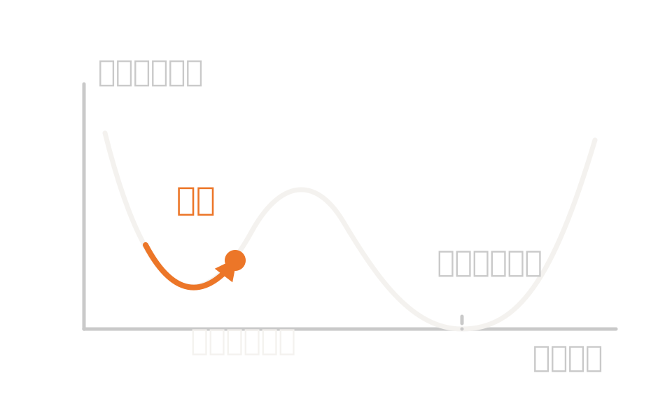
Diagram showing the merit function falling as design variables move, converging into a local valley

What the method is

Turn the target into a number and move the variables

Optimization in OpticStudio needs three things: a valid system that can be ray traced, variables specified, and a merit function. It only runs once all three are in place.

The merit function is a number expressing how close the optical system is to the targets set. It is defined as a quantity proportional to the square root of the weighted sum of the squared differences between each operand’s actual and target values. Operands fall into many categories: aberrations, MTF, point spread, encircled energy, real and paraxial ray quantities, constraints on lens data and more.

Variables are specified by placing a variable solve on the relevant cell. Curvature, thickness, glass, conic constant, parameter data, extra data and multi-configuration numeric data are all eligible.

How it works

Search the variables while evaluating the merit function

Two algorithms are available for local optimization. Damped least squares finds the descent direction from numerical derivatives of the merit function. Orthogonal descent lowers the value by orthogonalizing the variables and sampling the solution space discretely. The latter computes no numerical derivatives, which helps where the merit function is noisy and imprecise.

Local optimization looks for a local minimum. Where the design form itself has to change, a broad search is provided. That search builds and evaluates a variety of combinations within a defined range and saves the best candidates. It also has a mechanism for keeping diversity by rejecting designs that are too similar. What that stage is for is finding promising design forms; converging accurately on the best solution for each form is the job of a different algorithm.

Merit functionA quantity proportional to the square root of the weighted sum of the squared differences between each operand’s actual and target values. Build a default function with the wizard and add the operands you need.
VariablesPlace a variable solve on the cells you want as variables. Curvature, thickness, glass, conic constant, parameter data, extra data and multi-configuration numeric data are eligible.
Local searchMove the variables toward a local minimum with damped least squares or orthogonal descent.
Searching design formsBuild and evaluate a variety of designs within a defined range and save the best candidates. Then move on to refining the ones you choose.

Strengths of this method

Why this method is chosen

Many requirements on one scale

Requirements of different kinds, from aberrations and imaging performance to geometric constraints and coating and polarization quantities, all go into the same function as weighted operands.

An algorithm to suit the job

There is a method that finds the descent direction from numerical derivatives, and one that lowers the value without derivatives by orthogonalization and discrete sampling. The latter has the advantage in illumination design, where detector pixels make the merit function discontinuous.

A procedure that reaches design forms too

As well as local convergence, there is a search that gathers promising design forms broadly and a stage for choosing one or two and refining them. Discrete variables such as glass substitution are handled at that stage.

Where it fits

Where it fits, and where it does not

Where it is a good fit

→ when you have a reasonable starting point and want to bring aberrations or imaging performance toward a target

→ when you want to weight several requirements together and trade them off

→ when you want to specify a spatial frequency and design imaging contrast toward a target

→ when you want to settle geometry against a target distribution on a detector, as in an illumination system

→ when you want to gather candidates broadly in order to reconsider the design form itself

Where another method is the better fit

When you want to know the effect of manufacturing variation: this capability moves design variables to improve the nominal design. Finding how far machining and assembly variation degrade performance, and what range is acceptable, is the job of tolerance analysis. That said, this capability is used within tolerance analysis to settle the optimum values of compensators.

When you need a guarantee of optimality: a broad search rarely finds the global optimum on its own. Nor is there a known method for deciding, for a general optimization problem, whether a lower minimum exists once a local minimum has been reached. This capability is a search; it does not guarantee optimality.

When the starting point is not valid: local optimization only works once there is a valid starting point that can be ray traced. If the number of surfaces, the stop position and the initial glasses are unsettled, the skeleton of the design has to be decided first.

When the merit function does not express the requirement: a converged result is only what the merit function expresses. Without boundary conditions it can converge on thicknesses or curvatures that cannot be manufactured.

Applications

Typical applications

Imaging lens design

From singlets to multi-group lenses, refine the design against spot radius or wavefront criteria.

Designing toward a contrast target

Specify the spatial frequency of interest and improve imaging contrast by bringing the wavefront difference toward a target.

Illumination system optimization

Use operands that evaluate the distribution on a detector and settle geometry with the derivative-free method.

Glass substitution

Substitute glasses from a catalogue for those marked for substitution, and explore combinations with the broad search.

Inputs and outputs

What you provide, and what you get

INPUT

Starting system Design data in a state that can be ray traced, with fields and wavelengths
Variables Cells with a variable solve placed on them: curvature, thickness, glass, conic constant, parameter data, extra data, multi-configuration numeric data
Merit function The default function built by the wizard (type, criterion, reference point, pupil integration method), plus operands, targets and weights added by hand
Boundary conditions Upper and lower limits on glass and air thicknesses, and boundary operands giving upper limits, lower limits and targets
Run conditions Choice of algorithm, number of cycles, number of cores used

OUTPUT

Updated design Design data with the variable values updated
Merit function value Its progress during the run, and the final value
Candidate designs In a broad search, you specify how many to keep and the best candidates are saved as individual files
Re-evaluation results The usual analysis results for the updated design: spot, imaging performance, wavefront, transmittance and so on

How it works

How it works in practice

01

Specify the variables

Place a variable solve on the cells you want as degrees of freedom. Start with curvature and thickness and extend to conic constants and parameter data as needed.

02

Build the merit function

Build the default function with the wizard and choose the type, criterion, reference point and pupil integration method. Give the boundary values for glass and air thickness here too.

03

Run local optimization

Choose the algorithm and the number of cycles and run. Choosing automatic runs until progress stops.

04

Search design forms if needed

Where the design form itself has to change, or glasses are being substituted, gather candidates with the broad search and move on to refining the promising ones.

What decides the result is how the merit function is built. Without boundary conditions it can converge on geometry that cannot be manufactured. Where glass substitution is included, the merit function jumps discontinuously each time a glass changes, so use the broad search rather than local optimization.

Relationship to related methods

Division of roles and coupling with related analysis methods

Method Relationship Main targets When to use which
Optical optimization (this method) This method Bringing the nominal design toward its target Builds a merit function and moves the specified variables to lower it. There are two stages: local convergence, and the search for design forms.
Sequential Ray Tracing Upstream The evaluation itself The contents of the merit function are quantities obtained from this trace. A system that can be traced is the premise.
Tolerance Analysis Downstream Robustness to manufacturing variation Once the design is settled, apply machining and assembly variation, evaluate the degradation and find the acceptable range. This capability is used to settle compensator values.
Non-Sequential Ray Tracing Complementary Illumination and stray light systems For systems evaluated on a detector distribution, optimize with those trace results as operands.

View all analysis technologies →

Supporting products

Products that provide this method

Commercial software used for the design and analysis of imaging, illumination and laser systems. Alongside merit-function optimization it provides ray tracing, imaging performance evaluation and tolerance analysis in the same environment. See here for licensing, system requirements and deployment.

Ansys Zemax OpticStudio

View the product page →

FAQ

Frequently asked questions

How do I choose between the two algorithms?Damped least squares finds the descent direction from numerical derivatives of the merit function and is generally recommended for imaging systems. Orthogonal descent orthogonalizes the variables and samples the solution space discretely, computing no numerical derivatives. It has the advantage where detector pixels make the merit function discontinuous.
Will I get the global optimum?It is not guaranteed. A broad search rarely finds the global optimum on its own, and there is no known method for deciding, for a general optimization problem, whether a lower minimum exists once a local minimum has been reached. In practice you gather candidates broadly and then refine one or two.
How does this differ from tolerance analysis?The purposes differ. This capability moves design variables to improve the nominal design. Tolerance analysis applies a range of machining and assembly variation, evaluates the degradation and finds the acceptable tolerances. They are separate tasks, though this capability is used within tolerance analysis to find the optimum compensator values.
What can be a variable?Curvature, thickness, glass, conic constant, parameter data, extra data and multi-configuration numeric data. They are specified by placing a variable solve on the cell. Coating layer coefficients and index corrections can also be constrained with boundary operands.

References

Last updated

2026-08-19

Technical review

LightBridge Technical Support

Sources consulted

Ansys Zemax OpticStudio User Guide: Optimization OverviewAnsys Zemax OpticStudio User Guide: OptimizeAnsys Zemax OpticStudio User Guide: Optimization WizardAnsys Zemax OpticStudio User Guide: Global OptimizationAnsys Zemax OpticStudio User Guide: The Global Optimization AlgorithmAnsys Zemax OpticStudio User Guide: Hammer OptimizerAnsys Zemax OpticStudio User Guide: Optimization Operands by CategoryAnsys Zemax OpticStudio User Guide: Tolerancing OverviewAnsys Optics: How to design a singlet lens, Part 3: OptimizationAnsys Optics: How to optimize non-sequential optical systemsAnsys Optics: Optimizing for MTF performance using Contrast Optimization

We can advise on how to approach optical design optimization

Tell us the aim of the design and the specification you need to hold, and we will start from how to build the merit function.