
Home/Analysis Technologies/Thermal analysis/HEAT

Analysis Technologies | Thermal Analysis

HEAT (Thermal Conduction Analysis)

A method that solves the heat conduction equation by the finite-element method to obtain the temperature distribution within a structure, and passes that temperature to optical analysis to evaluate thermo-optic effects.

Target

Temperature field within a structure

Analysis type

Steady state, transient

Supporting products

Lumerical Multiphysics
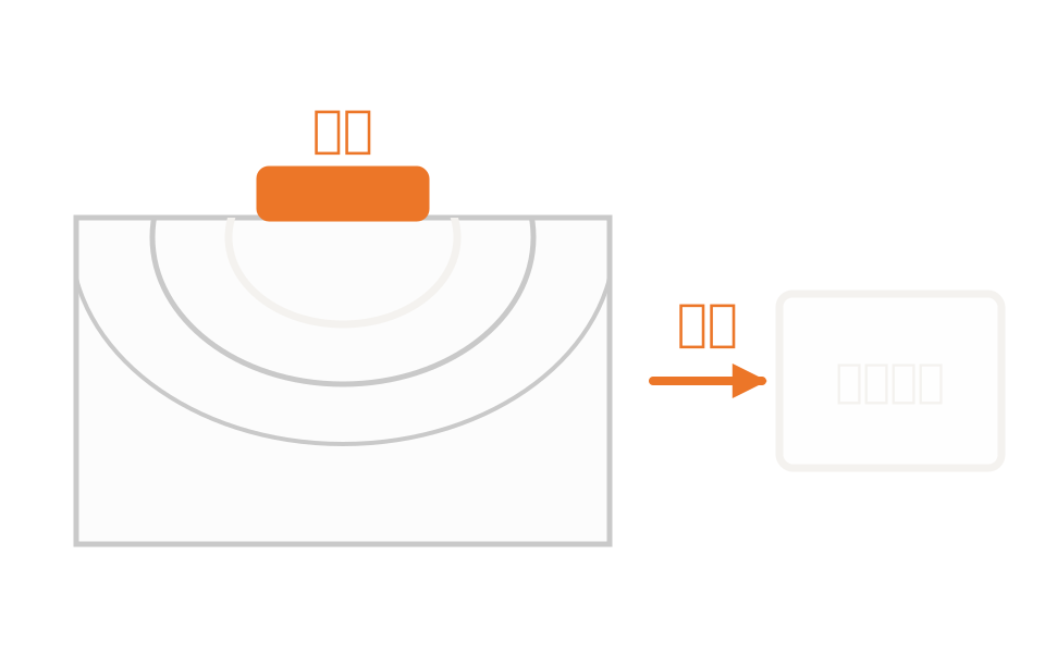
Schematic of the temperature distribution and heat flow with a heater as the source, and how that temperature is passed to the optical solver

What the method is

Solve the temperature, then carry it through to the change in optical properties

From heat sources and boundary conditions, obtain the temperature distribution within the structure. The subject is heat conduction in solids; fluids themselves are not solved. The material inputs are density, specific heat and thermal conductivity, plus electrical conductivity where electrical conduction is included. Both steady state and transient can be handled, so as well as the absolute temperature you can evaluate the time taken to reach steady state.

Coupling with electrical conduction happens inside the solution. There is a mode that solves heat conduction alone and an electro-thermal mode that includes electrical conduction; in the latter, Joule heating from the current enters the heat conduction equation as a source and heat and electrical conduction are solved self-consistently. That is the basic arrangement when self-heating has to be included for a high-current device.

What this method solves stops at the temperature field. The change in optical properties is evaluated by passing the temperature distribution to the optical analysis as temperature data, updating the refractive index through a temperature-dependent index model, and re-solving. The handover is one-way: optical results do not return to the temperature solution. In other words, the thermal and optical coupling is not self-consistent.

How it works

Solving heat flow element by element

Heat conduction analysis is the problem of solving one partial differential equation for temperature. Heat capacity per unit volume times the rate of change of temperature, the inflow and outflow by conduction, and the heat source: the temperature distribution sought is the one that balances those three across the whole region.

Dividing the region into finite elements and representing temperature by values at mesh nodes turns the continuous problem into algebraic equations in a finite number of unknowns. The finer the elements the more precise the solution, and the greater the cost.

For steady state, the form with the time-derivative term dropped is solved. For transient, time is discretized too, and the time step is adjusted against a tolerance on the local truncation error. In either case the formulation presumes the timescale of interest is much longer than the relaxation time of the material.

Governing equationsSolves the balance between heat capacity times the rate of change of temperature, transport by conduction, and the heat source. In steady state the time-derivative term drops out.
DiscretizationThe structure is divided into a finite-element mesh and the temperature obtained at the mesh nodes. Finer elements raise accuracy and cost.
Boundary conditionsFixed temperature, heat generation, heat flux, convection, radiation and adiabatic conditions are given per surface. Radiation is evaluated from emissivity and ambient temperature, convection from the heat transfer coefficient and ambient temperature.
The quasi-static assumptionThe timescale of interest is presumed to be much longer than the relaxation time of the material. Heat transport faster than that is outside this formulation.

Strengths of this method

Why this method is chosen

Heat removal specified as you need it

Fixed temperature, heat flux, convection and radiation can be combined per surface, so the heat removal path can be represented close to the real assembly.

Steady state and transient from one model

From one structural description you can obtain both the steady-state temperature distribution and the time variation of temperature during switching. The response time constant comes from this too.

Heat generation and electrical conduction solved together

Because heating from electrical conduction can be treated self-consistently as a source, self-heating is evaluated without relying on post-processing.

Where it fits

Where it fits, and where it does not

Where it is a good fit

→ when you are designing a thermo-optic phase shifter driven by a heater

→ when you want to estimate the resonant wavelength shift from self-heating

→ when you want to evaluate thermal crosstalk between densely packed components

→ when you need the temperature time constant for switching

→ when you want the temperature rise from heating by optical absorption or current

Where another method is the better fit

You want to solve the flow: fluids themselves are not solved. A fluid only serves to provide a boundary condition, so where the flow field is the question, that is the territory of thermal-fluid analysis.

Carrier transport in semiconductors: where the current is set by carrier transport in a semiconductor, couple heat on the drift-diffusion side. The electrical treatment here goes as far as conduction in a conductor.

Optical response alone: if you only need optical response with no temperature change, electromagnetic or mode analysis is enough on its own.

Stress and deformation: evaluating mechanical stress and deformation is the territory of structural analysis tools.

Applications

Typical applications

Silicon Photonics

Used for thermo-optic phase shifters and wavelength control of ring resonators.

Optical transceivers and CPO

Evaluate thermal crosstalk between densely packed components.

Lasers and optical amplifiers

Estimate the drift in characteristics caused by self-heating.

Infrared sensors

Evaluate the temperature rise from optical absorption in devices such as metamaterial bolometers.

Inputs and outputs

What you provide, and what you get

INPUT

Structure The layer stack, with materials assigned per region
Material properties Density, specific heat and thermal conductivity, plus electrical conductivity where electrical conduction is included
Heat sources Uniform heat generation, or heat generation or charge data imported from another analysis
Boundary conditions Fixed temperature, heat generation, heat flux, convection, radiation, adiabatic

OUTPUT

Temperature distribution Temperature field within a structure
Heat flow Heat flow from the power flow monitor
Transient response The time variation of temperature and the time constant to reach steady state
Handover data Temperature data passed to optical analysis, used together with a temperature-dependent index model

How it works

How it works in practice

01

Specify the thermal properties of the materials

Give density, specific heat and thermal conductivity. Solids and fluids are defined separately. Specify electrical conductivity too if electrical conduction is included.

02

Build the geometry and assign materials

Set the extent so that the heat sources and the heat removal path lie inside the analysis region. Leaving out the substrate or the assembly makes the temperature come out too high.

03

Settle the analysis type and the scope of the physics

Choose steady state or transient, and whether to solve heat conduction alone or include electrical conduction. The mesh is set here too.

04

Set boundary conditions and monitors, and run

Give fixed temperature, heat generation, heat flux, convection, radiation and adiabatic conditions per surface, and place temperature and power flow monitors.

How you choose the boundary conditions decides the temperature distribution more than the amount of heat generated. Note also that the convection condition is intended for steady state. Step 04 is where most of your time should go.

Relationship to related methods

Division of roles and coupling with related analysis methods

Method Relationship Main targets When to use which
HEAT (this method) This method Temperature distribution within a structure Solves the heat conduction equation by the finite-element method for the temperature field and heat flow. It does not obtain the change in optical properties.
CHARGE Coupling Carrier transport in semiconductors Where the current is set by carrier transport in a semiconductor, heat is coupled self-consistently on that side.
FDTD Upstream Optical absorption distribution Receives the heat generation distribution obtained from absorption as a source.
FEEM Downstream Cross-sectional modes after a temperature change The temperature obtained is passed across, and the change in effective index is obtained there through a temperature-dependent index model.
MQW Downstream Quantum well gain The recipient when temperature is passed as a single scalar value. The temperature distribution within the well is not reflected.

View all analysis technologies →

Supporting products

Products that provide this method

A commercial software environment providing heat conduction analysis. Electrical and quantum well analysis sit alongside it, and the handover of data to optical analysis happens there too. See here for licensing, system requirements and deployment.

Lumerical Multiphysics

View the product page →

FAQ

Frequently asked questions

What does transient analysis give?The time from switching the heater on until the temperature reaches steady state, which is the response speed of a thermo-optic phase shifter. The time step is adjusted against a tolerance on the local truncation error.
Can it handle heating from optical absorption?Yes. The absorption distribution obtained from electromagnetic analysis is imported as a heat source. A heat source object is provided for importing heat generation or charge data.
How is temperature reflected in the optical analysis?The temperature distribution is passed to the optical analysis as temperature data, and the refractive index is updated through a temperature-dependent index model. The default is a linear model around a reference temperature, and a table of index against temperature can be supplied if needed. The handover is one-way.
How much should I model?As far as the heat removal path. Leaving out the substrate or the assembly makes the temperature come out too high. Choose the convection and radiation conditions to match the real assembly too.

References

Last updated

2026-08-18

Technical review

LightBridge Technical Support

Sources consulted

Ansys Optics: HEAT solver introductionAnsys Optics: HEAT solver – Simulation objectAnsys Optics: HEAT product reference manualAnsys Optics: Boundary Conditions in HEAT – Simulation ObjectAnsys Optics: Temperature dependent refractive index modelsAnsys Optics: Thermal phase shifter workflow

We can advise where thermal effects are a concern

Tell us the structure and the characteristics you want to evaluate, and we will propose the method and product that suit.